Exercise Week 8: Solutions

library(fpp3)
library(patchwork)

fpp3 9.11, Ex1

Figure 9.32 shows the ACFs for 36 random numbers, 360 random numbers and 1,000 random numbers.

Explain the differences among these figures. Do they all indicate that the data are white noise?

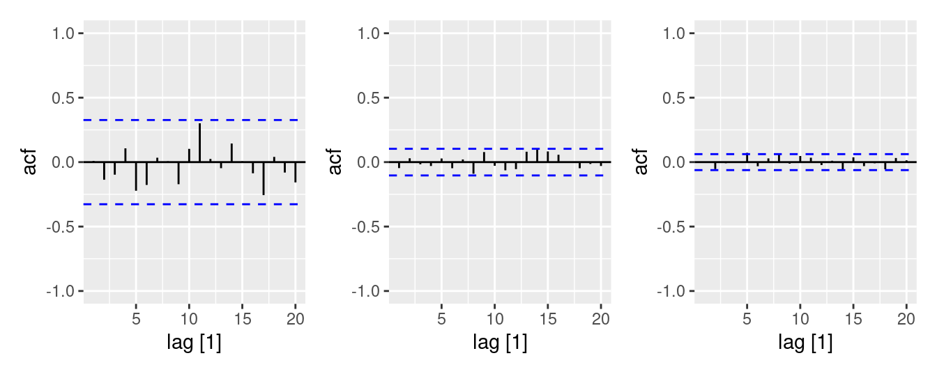
Left: ACF for a white noise series of 36 numbers. Middle: ACF for a white noise series of 360 numbers. Right: ACF for a white noise series of 1,000 numbers.

The figures show different critical values (blue dashed lines).
All figures indicate that the data is white noise.

Why are the critical values at different distances from the mean of zero? Why are the autocorrelations different in each figure when they each refer to white noise?

The critical values are at different distances from zero because the data sets have different number of observations. The more observations in a data set, the less noise appears in the correlation estimates (spikes). Therefore the critical values for bigger data sets can be smaller in order to check if the data is not white noise.

fpp3 9.11, Ex2

A classic example of a non-stationary series are stock prices. Plot the daily closing prices for Amazon stock (contained in gafa_stock), along with the ACF and PACF. Explain how each plot shows that the series is non-stationary and should be differenced.

gafa_stock |>
  filter(Symbol == "AMZN") |>
  mutate(t = row_number()) |>
  update_tsibble(index = t) |>
  gg_tsdisplay(Close, plot_type = "partial")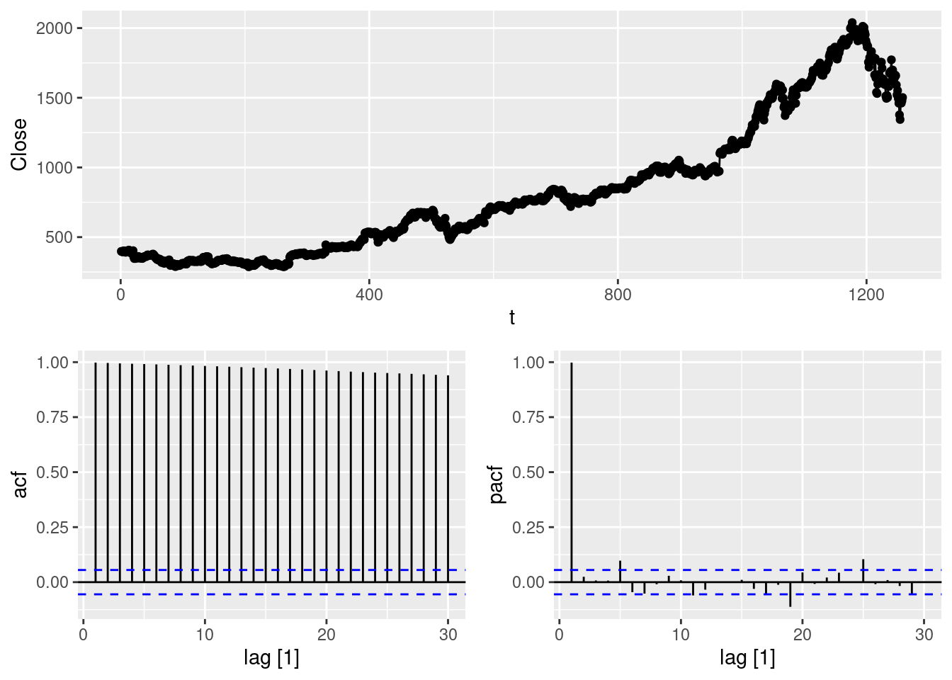

The time plot shows the series “wandering around”, which is a typical indication of non-stationarity. Differencing the series should remove this feature.

ACF does not drop quickly to zero, moreover the value r_1 is large and positive (almost 1 in this case). All these are signs of a non-stationary time series. Therefore it should be differenced to obtain a stationary series.

PACF value r_1 is almost 1. All other values r_i, i>1 are small. This is a sign of a non-stationary process that should be differenced in order to obtain a stationary series.

fpp3 9.11, Ex3

For the following series, find an appropriate Box-Cox transformation and order of differencing in order to obtain stationary data.

Turkish GDP from global_economy.

turkey <- global_economy |> filter(Country == "Turkey")
turkey |> autoplot(GDP)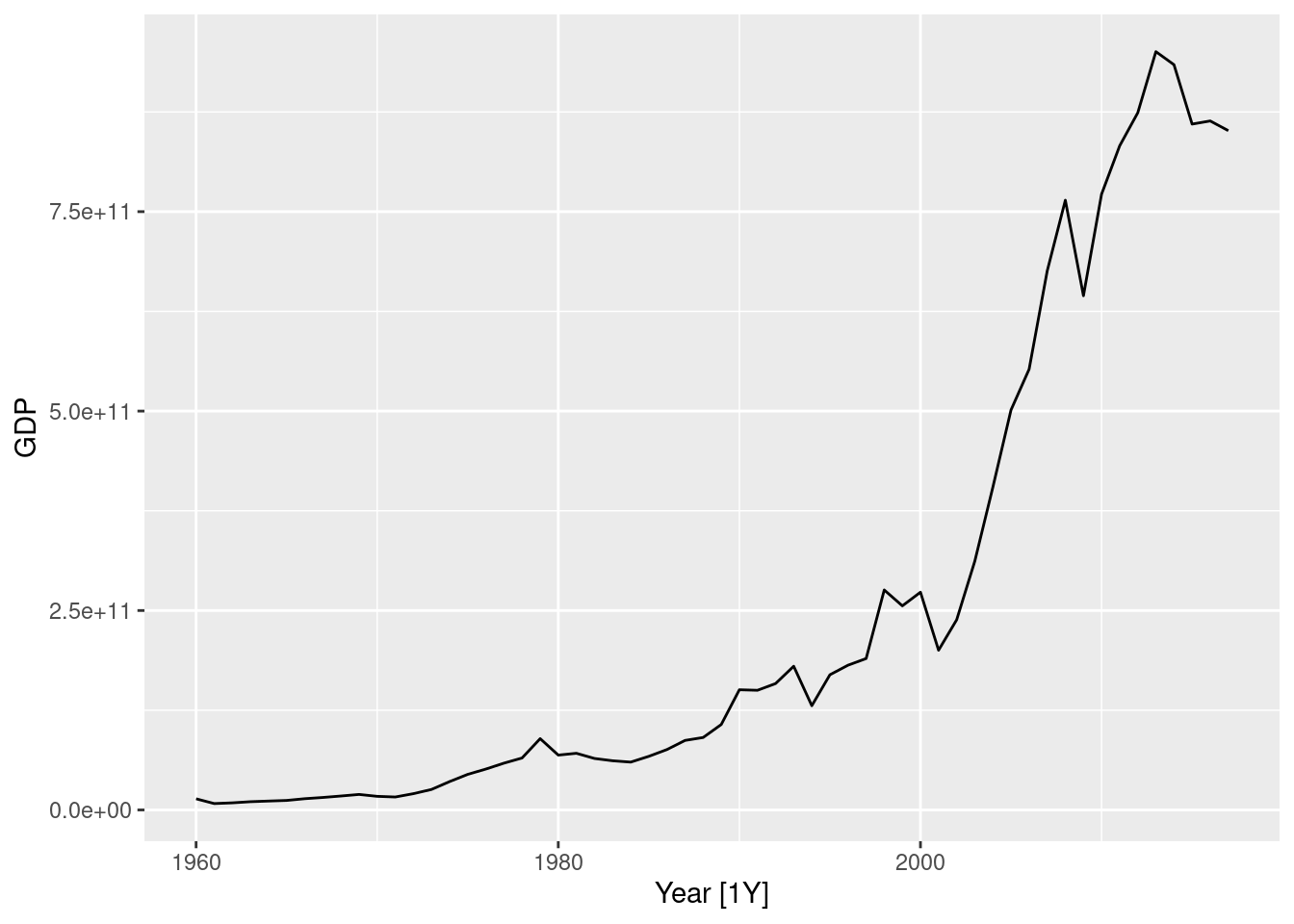

turkey |> autoplot(log(GDP))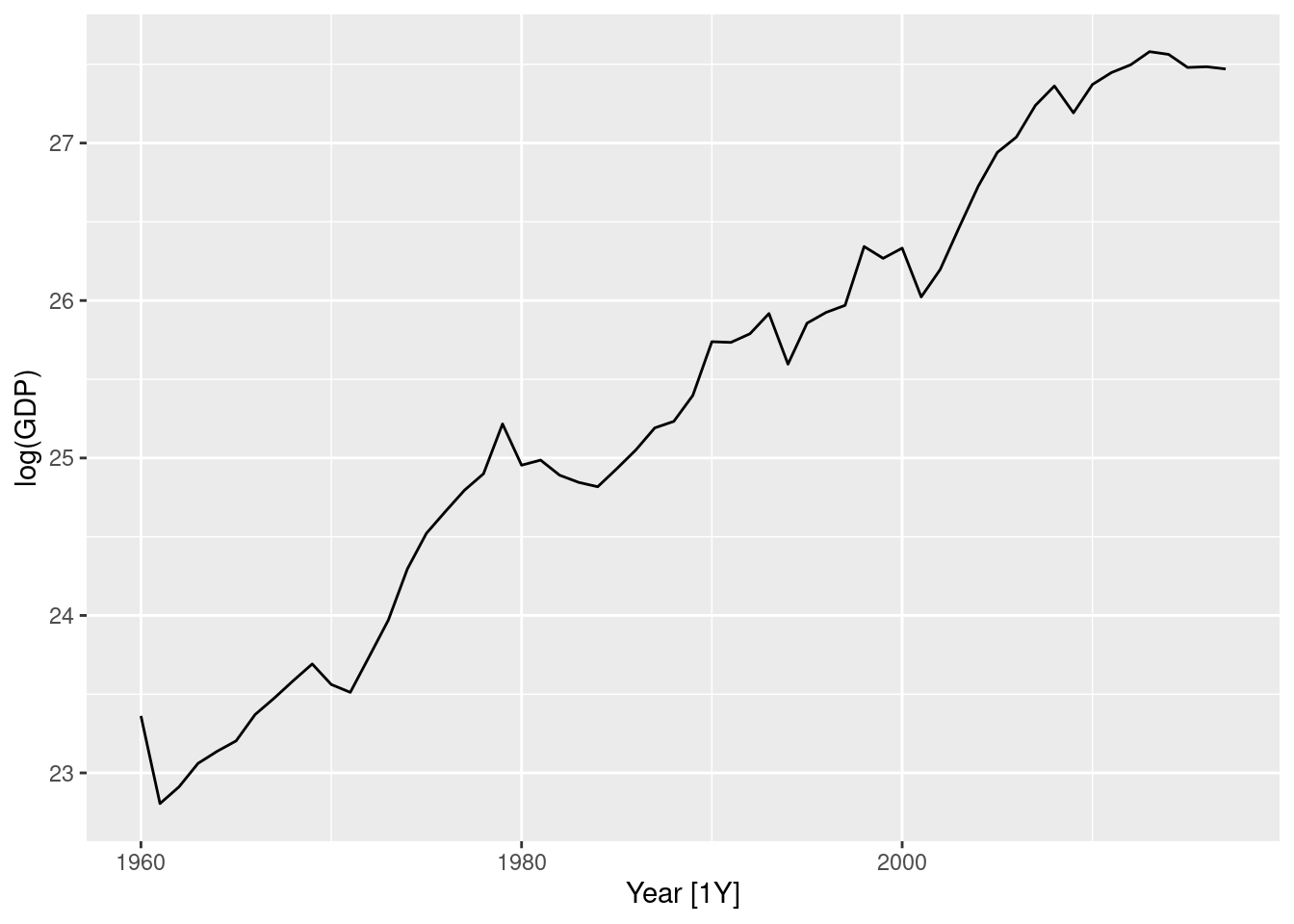

turkey |> autoplot(log(GDP) |> difference())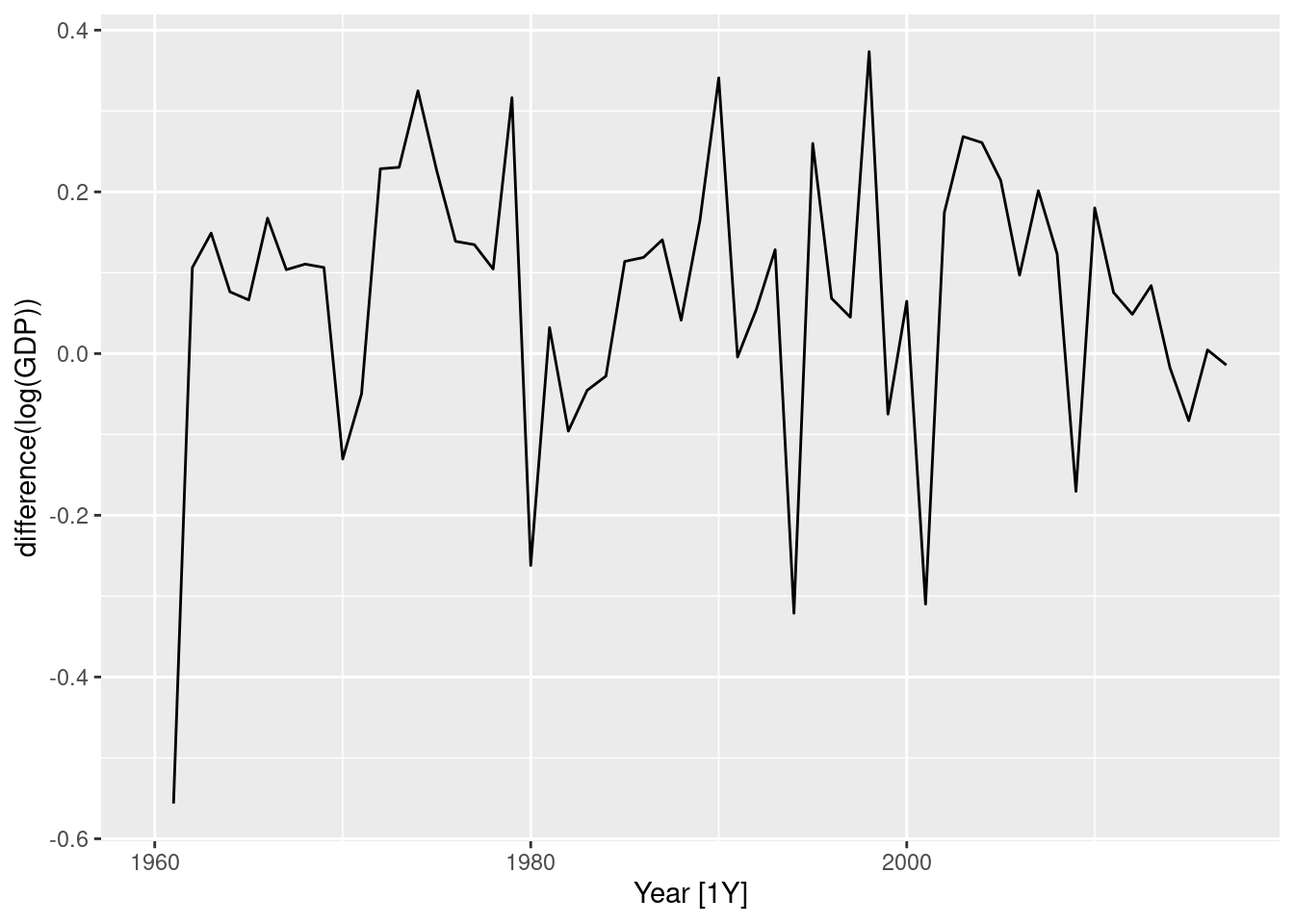

turkey |> features(GDP, guerrero)

# A tibble: 1 × 2
  Country lambda_guerrero
  <fct>             <dbl>
1 Turkey            0.157

Logs and differences make the data appear stationary.
Using a Box-Cox transformation with \lambda between 0 and 0.2 would also have worked well.

Accommodation takings in the state of Tasmania from aus_accommodation.

tas <- aus_accommodation |> filter(State == "Tasmania")
tas |> autoplot(Takings)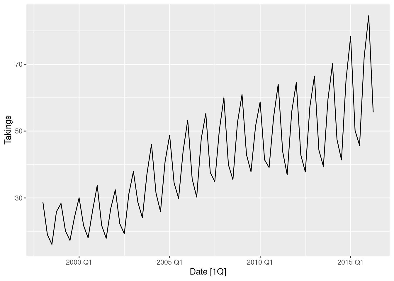

tas |> autoplot(log(Takings))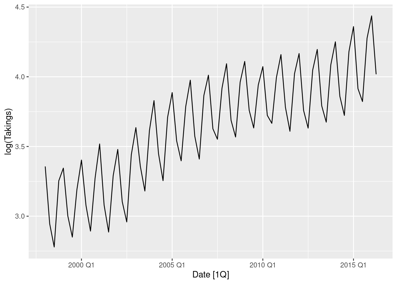

tas |> autoplot(log(Takings) |> difference(lag = 12))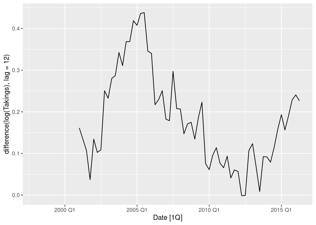

tas |> autoplot(log(Takings) |> difference(lag = 12) |> difference())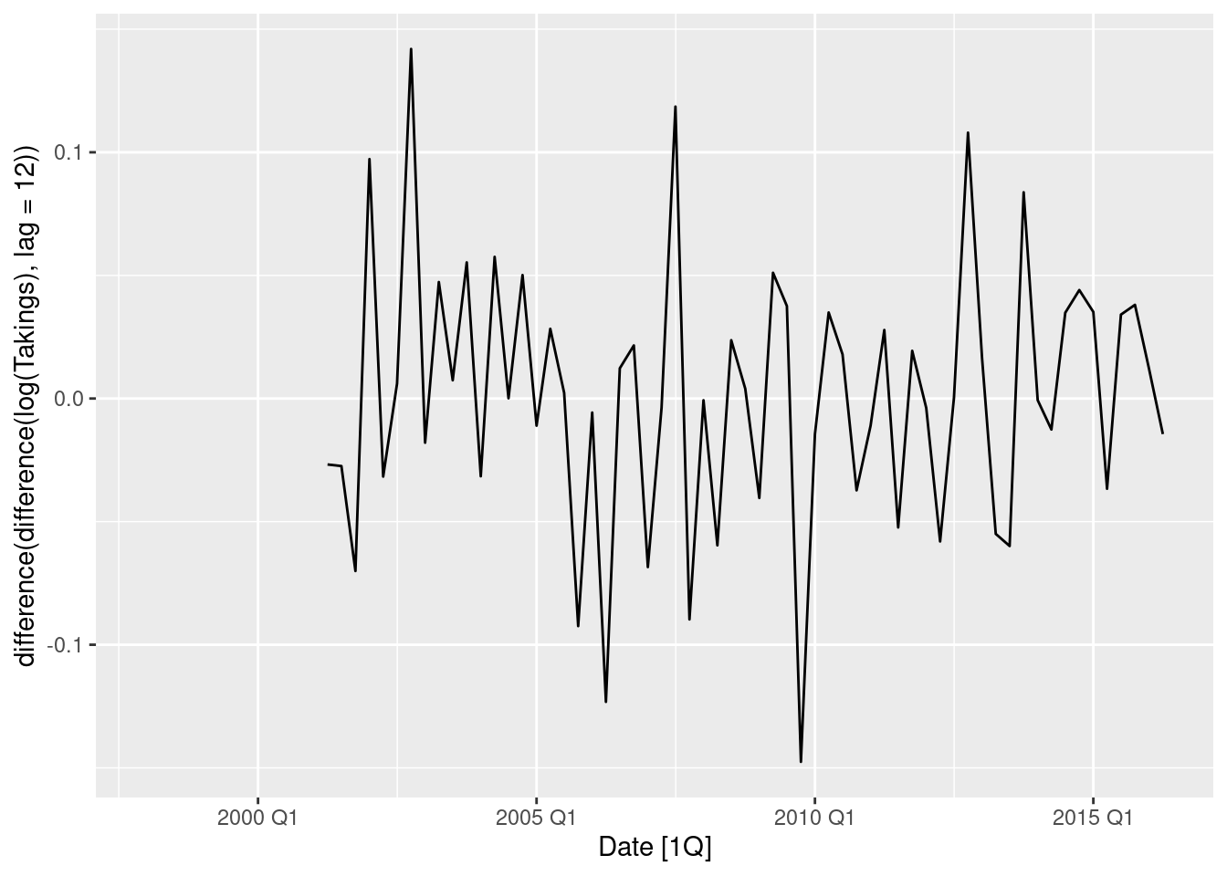

tas |> features(Takings, guerrero)

# A tibble: 1 × 2
  State    lambda_guerrero
  <chr>              <dbl>
1 Tasmania         0.00182

Logs followed by seasonal and first differences make the data appear stationary.
The automatically selected Box-Cox \lambda value is very close to zero, confirming the choice of using logs.

Monthly sales from souvenirs.

souvenirs |> autoplot(Sales)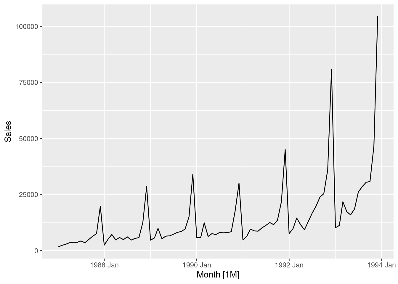

souvenirs |> autoplot(log(Sales))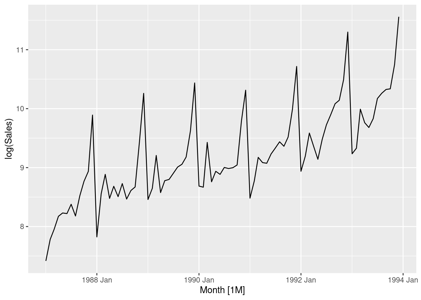

souvenirs |> autoplot(log(Sales) |> difference(lag=12))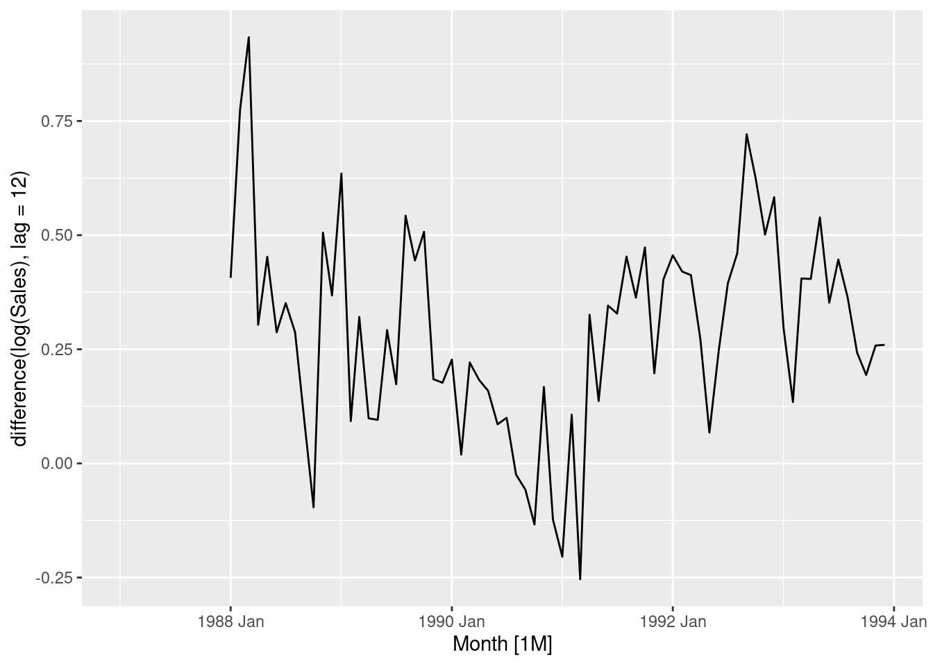

souvenirs |> autoplot(log(Sales) |> difference(lag=12) |> difference())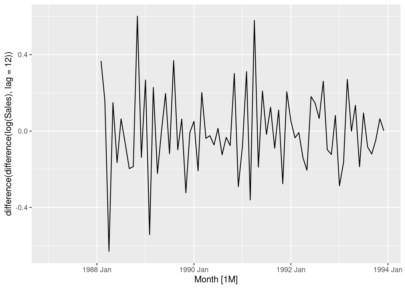

souvenirs |> features(Sales, guerrero)

# A tibble: 1 × 1
  lambda_guerrero
            <dbl>
1         0.00212

Logs followed by seasonal and first differences make the data appear stationary.
The automatically selected Box-Cox \lambda value is very close to zero, confirming the choice of using logs.

fpp3 9.11, Ex4

For the souvenirs data, write down the differences you chose above using backshift operator notation.

Let y_t = log(Sales). Then (1-B^{12})(1-B)y_t gives the differences used above.

fpp3 9.11, Ex5

For your retail data (from Exercise 8 in Section 2.10), find the appropriate order of differencing (after transformation if necessary) to obtain stationary data.

set.seed(12345678)
myseries <- aus_retail |>
  filter(
    `Series ID` == sample(aus_retail$`Series ID`, 1),
    Month < yearmonth("2018 Jan")
  )
myseries |> autoplot(Turnover)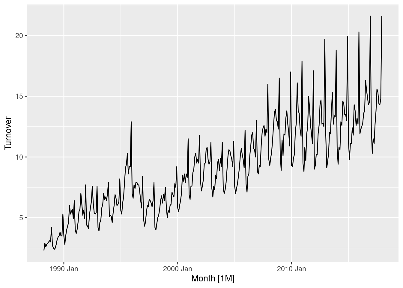

Data requires a transformation as the variation is proportional to the level of the series. A log transformation will be okay, although it does seem to be too strong.

myseries |> autoplot(log(Turnover))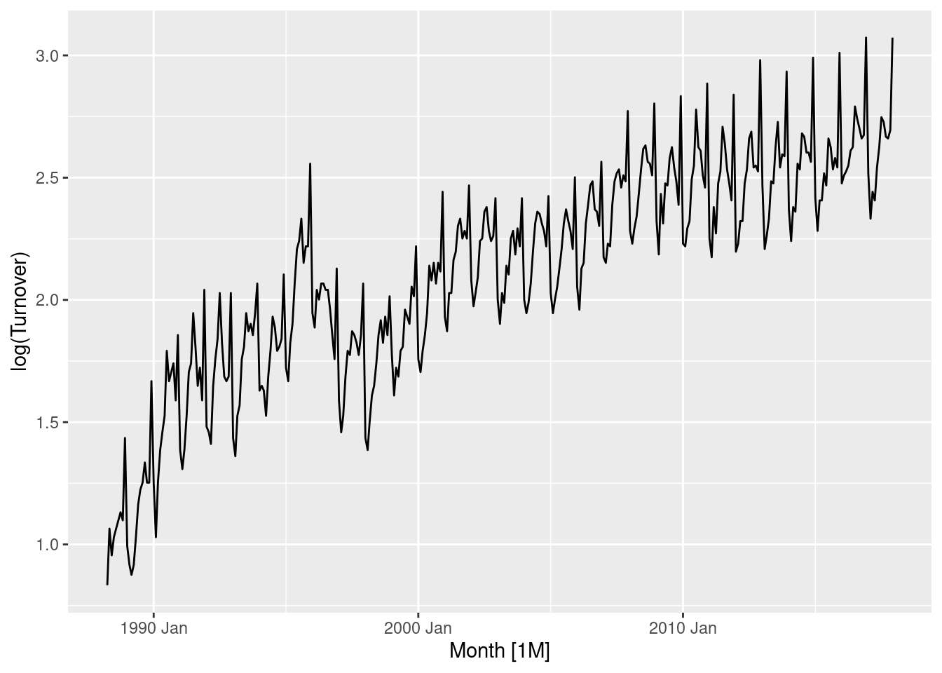

Data contains seasonality, so a seasonal difference is required.

myseries |> autoplot(log(Turnover) |> difference(lag = 12))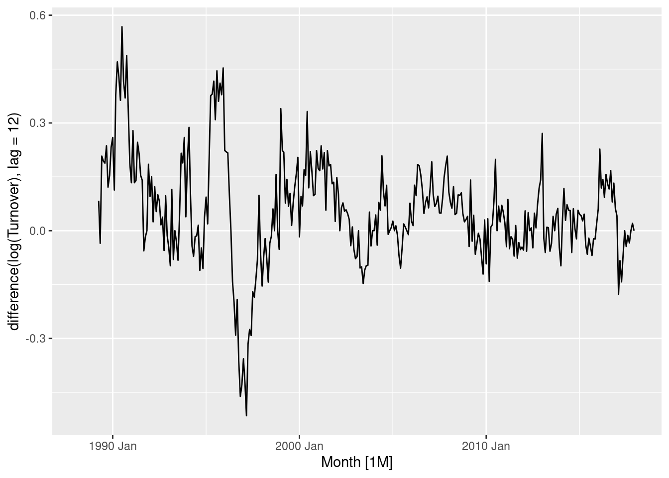

Data still appears to have extended periods of high values and low values. A first order differencing may be useful.

myseries |> autoplot(log(Turnover) |> difference(lag = 12) |> difference())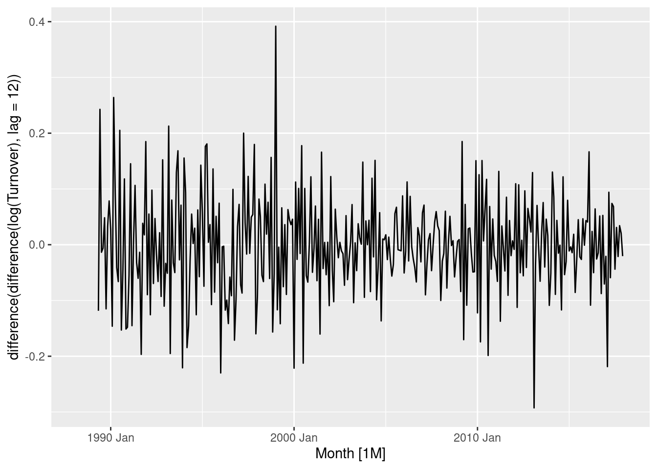

The dataset is now clearly stationary. Either just a seasonal difference, or both a seasonal and first difference, could be used here.