Exercise Week 7: Solutions

library(fpp3)

fpp3 8.8, Ex5

Data set global_economy contains the annual Exports from many countries. Select one country to analyse.

Plot the Exports series and discuss the main features of the data.

global_economy |>
  filter(Country == "Argentina") |>
  autoplot(Exports)

There is a huge jump in Exports in 2002, due to the deregulation of the Argentinian peso. Since then, Exports (as a percentage of GDP) has gradually returned to 1990 levels.

Use an ETS(A,N,N) model to forecast the series, and plot the forecasts.

etsANN <- global_economy |>
  filter(Country == "Argentina") |>
  model(ETS(Exports ~ error("A") + trend("N") + season("N")))
etsANN |>
  forecast(h = 10) |>
  autoplot(global_economy)

Compute the RMSE values for the training data.

accuracy(etsANN) |> select(RMSE)

# A tibble: 1 × 1
   RMSE
  <dbl>
1  2.78

Compare the results to those from an ETS(A,A,N) model. (Remember that the trended model is using one more parameter than the simpler model.) Discuss the merits of the two forecasting methods for this data set.

fit <- global_economy |>
  filter(Country == "Argentina") |>
  model(
    ses = ETS(Exports ~ error("A") + trend("N") + season("N")),
    holt = ETS(Exports ~ error("A") + trend("A") + season("N"))
  )
accuracy(fit)

# A tibble: 2 × 11
  Country   .model .type         ME  RMSE   MAE   MPE  MAPE  MASE RMSSE    ACF1
  <fct>     <chr>  <chr>      <dbl> <dbl> <dbl> <dbl> <dbl> <dbl> <dbl>   <dbl>
1 Argentina ses    Training 0.0762   2.78  1.62 -1.73  15.7 0.983 0.986 0.00902
2 Argentina holt   Training 0.00795  2.78  1.64 -2.51  15.9 0.994 0.986 0.0271

There is very little difference in training RMSE between these models. So the extra parameter is not doing much.

Compare the forecasts from both methods. Which do you think is best?

fit |>
  forecast(h = 10) |>
  autoplot(global_economy)

The forecasts are similar. In this case, the simpler model is preferred.

Calculate a 95% prediction interval for the first forecast for each series, using the RMSE values and assuming normal errors. Compare your intervals with those produced using R.

standard error. (from RMSE)
mean (from forecast)

s <- accuracy(fit) |> pull(RMSE)
yhat <- forecast(fit, h = 1) |> pull(.mean)
# SES
yhat[1] + c(-1, 1) * qnorm(0.975) * s[1]

[1]  5.882074 16.764136

# Holt
yhat[2] + c(-1, 1) * qnorm(0.975) * s[2]

[1]  5.989515 16.872908

fit |>
  forecast(h = 1) |>
  mutate(PI = hilo(Exports, level = 95))

# A fable: 2 x 6 [1Y]
# Key:     Country, .model [2]
  Country   .model  Year    Exports .mean                     PI
  <fct>     <chr>  <dbl>     <dist> <dbl>                 <hilo>
1 Argentina ses     2018   N(11, 8)  11.3 [5.785765, 16.86044]95
2 Argentina holt    2018 N(11, 8.3)  11.4 [5.791571, 17.07085]95

Using RMSE yields narrower prediction interval while using the values from hilo() function gives wider prediction interval.
Using RMSE has failed to take account of the degrees of freedom for each model. Compare the following

sse <- augment(fit) |>
  as_tibble() |>
  group_by(.model) |>
  summarise(s = sum(.resid^2)) |>
  pull(s)

n <- global_economy |>
  filter(Country == "Argentina") |>
    nrow()

# sse method= alpha, level=> 2
# holt linear = alpha, level, trend, b => 4

s <- sqrt(sse / (n - c(2, 4)))

# SES
yhat[1] + c(-1, 1) * qnorm(0.975) * s[1]

[1]  5.785088 16.861122

# Holt
yhat[2] + c(-1, 1) * qnorm(0.975) * s[2]

[1]  5.79226 17.07016

fpp3 8.8, Ex6

Forecast the Chinese GDP from the global_economy data set using an ETS model. Experiment with the various options in the ETS() function to see how much the forecasts change with damped trend, or with a Box-Cox transformation. Try to develop an intuition of what each is doing to the forecasts.

[Hint: use h=20 when forecasting, so you can clearly see the differences between the various options when plotting the forecasts.]

china <- global_economy |>
  filter(Country == "China")
china |> autoplot(GDP)

It clearly needs a relatively strong transformation due to the increasing variance.

china |> autoplot(box_cox(GDP, 0.2))

china |> features(GDP, guerrero)

# A tibble: 1 × 2
  Country lambda_guerrero
  <fct>             <dbl>
1 China           -0.0345

Making \lambda=0.2 looks ok.
The Guerrero method suggests an even stronger transformation. Let’s also try a log.

fit <- china |>
  model(
    ets = ETS(GDP),
    ets_damped = ETS(GDP ~ trend("Ad")),
    ets_bc = ETS(box_cox(GDP, 0.2)),
    ets_log = ETS(log(GDP))
  )

fit

# A mable: 1 x 5
# Key:     Country [1]
  Country          ets    ets_damped       ets_bc      ets_log
  <fct>        <model>       <model>      <model>      <model>
1 China   <ETS(M,A,N)> <ETS(M,Ad,N)> <ETS(A,A,N)> <ETS(A,A,N)>

augment(fit)

# A tsibble: 232 x 7 [1Y]
# Key:       Country, .model [4]
   Country .model  Year          GDP      .fitted        .resid   .innov
   <fct>   <chr>  <dbl>        <dbl>        <dbl>         <dbl>    <dbl>
 1 China   ets     1960 59716467625. 49001691297.  10714776328.  0.219  
 2 China   ets     1961 50056868958. 66346643194. -16289774236. -0.246  
 3 China   ets     1962 47209359006. 51607368186.  -4398009180. -0.0852 
 4 China   ets     1963 50706799903. 47386494407.   3320305495.  0.0701 
 5 China   ets     1964 59708343489. 51919091574.   7789251914.  0.150  
 6 China   ets     1965 70436266147. 63350421234.   7085844913.  0.112  
 7 China   ets     1966 76720285970. 76289186599.    431099371.  0.00565
 8 China   ets     1967 72881631327. 82708375812.  -9826744486. -0.119  
 9 China   ets     1968 70846535056. 75804820984.  -4958285928. -0.0654 
10 China   ets     1969 79705906247. 72222259470.   7483646777.  0.104  
# ℹ 222 more rows

fit |>
  forecast(h = "20 years") |>
  autoplot(china, level = NULL)

The transformations have a big effect, with small lambda values creating big increases in the forecasts.
The damping has relatively a small effect.

fpp3 8.8, Ex7

Find an ETS model for the Gas data from aus_production and forecast the next few years. Why is multiplicative seasonality necessary here? Experiment with making the trend damped. Does it improve the forecasts?

aus_production |> autoplot(Gas)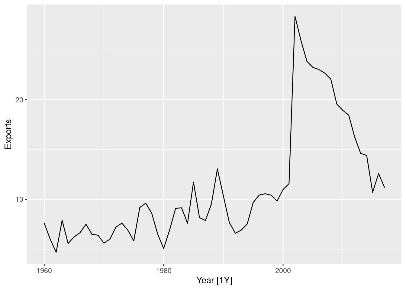

There is a huge increase in variance as the series increases in level. => That makes it necessary to use multiplicative seasonality.

fit <- aus_production |>
  model(
    hw = ETS(Gas ~ error("M") + trend("A") + season("M")),
    hwdamped = ETS(Gas ~ error("M") + trend("Ad") + season("M")),
  )

fit |> glance()

# A tibble: 2 × 9
  .model    sigma2 log_lik   AIC  AICc   BIC   MSE  AMSE    MAE
  <chr>      <dbl>   <dbl> <dbl> <dbl> <dbl> <dbl> <dbl>  <dbl>
1 hw       0.00324   -831. 1681. 1682. 1711.  21.1  32.2 0.0413
2 hwdamped 0.00329   -832. 1684. 1685. 1718.  21.1  32.0 0.0417

The non-damped model seems to be doing slightly better here, probably because the trend is very strong over most of the historical data.

fit |>
  select(hw) |>
  gg_tsresiduals()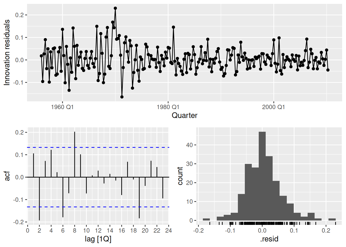

fit |> tidy()

# A tibble: 19 × 3
   .model   term  estimate
   <chr>    <chr>    <dbl>
 1 hw       alpha   0.653 
 2 hw       beta    0.144 
 3 hw       gamma   0.0978
 4 hw       l[0]    5.95  
 5 hw       b[0]    0.0706
 6 hw       s[0]    0.931 
 7 hw       s[-1]   1.18  
 8 hw       s[-2]   1.07  
 9 hw       s[-3]   0.816 
10 hwdamped alpha   0.649 
11 hwdamped beta    0.155 
12 hwdamped gamma   0.0937
13 hwdamped phi     0.980 
14 hwdamped l[0]    5.86  
15 hwdamped b[0]    0.0994
16 hwdamped s[0]    0.928 
17 hwdamped s[-1]   1.18  
18 hwdamped s[-2]   1.08  
19 hwdamped s[-3]   0.817

fit |>
  augment() |>
  filter(.model == "hw") |>
  features(.innov, ljung_box, lag = 24)

# A tibble: 1 × 3
  .model lb_stat lb_pvalue
  <chr>    <dbl>     <dbl>
1 hw        57.1  0.000161

There is still some small correlations left in the residuals, showing the model has not fully captured the available information.
There also appears to be some heteroskedasticity in the residuals with larger variance in the first half the series.

fit |>
  forecast(h = 36) |>
  filter(.model == "hw") |>
  autoplot(aus_production)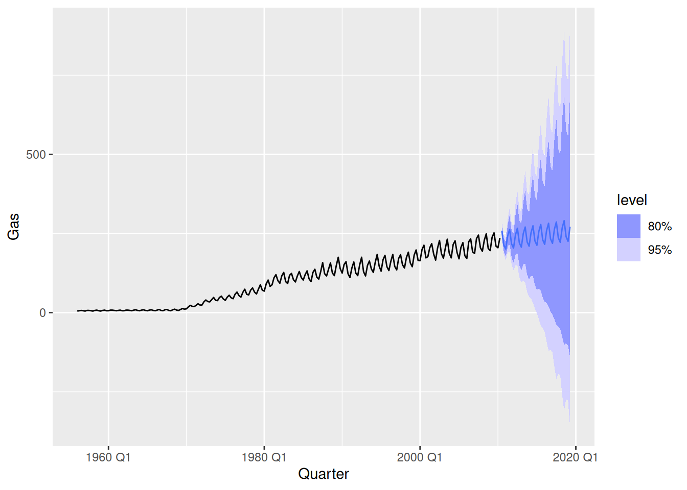

While the point forecasts look ok, the intervals are excessively wide.

fpp3 8.8, Ex8

Recall your retail time series data (from Exercise 6 in Section 2.10).

Why is multiplicative seasonality necessary for this series?

set.seed(12345678)
myseries <- aus_retail |>
  filter(`Series ID` == sample(aus_retail$`Series ID`, 1))
myseries |> autoplot(Turnover)

The variation in the seasonal pattern increases as the level of the series rises. (This may not be true for every series, but is true for almost all of them.)

Apply Holt-Winters’ multiplicative method to the data. Experiment with making the trend damped.

fit <- myseries |>
  model(
    hw = ETS(Turnover ~ error("M") + trend("A") + season("M")),
    hwdamped = ETS(Turnover ~ error("M") + trend("Ad") + season("M"))
  )
fc <- fit |> forecast(h = 36)
fc |> autoplot(myseries)

Compare the RMSE of the one-step forecasts from the two methods. Which do you prefer?

accuracy(fit)

# A tibble: 2 × 12
  State      Industry .model .type      ME  RMSE   MAE     MPE  MAPE  MASE RMSSE
  <chr>      <chr>    <chr>  <chr>   <dbl> <dbl> <dbl>   <dbl> <dbl> <dbl> <dbl>
1 Northern … Clothin… hw     Trai… -0.0128 0.613 0.450 -0.469   5.15 0.513 0.529
2 Northern … Clothin… hwdam… Trai…  0.0398 0.616 0.444 -0.0723  5.06 0.507 0.531
# ℹ 1 more variable: ACF1 <dbl>

The non-damped method is doing slightly better (on RMSE), but the damped method is doing better on most other scores. I’d be inclined to use the damped method here as the trend at the end of the series seems to be flattening.

Check that the residuals from the best method look like white noise.

fit |>
  select("hwdamped") |>
  gg_tsresiduals()

There are significant spikes at lags 8 and 18 in the ACF, but they are relatively small and probably of no consequence.

augment(fit) |>
  filter(.model == "hwdamped") |>
  features(.innov, ljung_box, lag = 36)

# A tibble: 1 × 5
  State              Industry                           .model lb_stat lb_pvalue
  <chr>              <chr>                              <chr>    <dbl>     <dbl>
1 Northern Territory Clothing, footwear and personal a… hwdam…    35.2     0.507

It seems that there is enough autocorrelation in the residuals for this to be significant. But in practice it will make little difference to the forecasts or prediction intervals.

Now find the test set RMSE, while training the model to the end of 2010. Can you beat the seasonal naïve approach from Exercise 7 in Section 5.10?

myseries |>
  filter(year(Month) < 2011) |>
  model(
    snaive = SNAIVE(Turnover),
    hw = ETS(Turnover ~ error("M") + trend("A") + season("M")),
    hwdamped = ETS(Turnover ~ error("M") + trend("Ad") + season("M"))
  ) |>
  forecast(h = "7 years") |>
  accuracy(myseries)

# A tibble: 3 × 12
  .model   State    Industry .type      ME  RMSE   MAE     MPE  MAPE  MASE RMSSE
  <chr>    <chr>    <chr>    <chr>   <dbl> <dbl> <dbl>   <dbl> <dbl> <dbl> <dbl>
1 hw       Norther… Clothin… Test  -1.45    1.71 1.51  -11.8   12.2  1.66  1.41 
2 hwdamped Norther… Clothin… Test   0.0290  1.13 0.846  -0.831  6.32 0.925 0.934
3 snaive   Norther… Clothin… Test   0.673   1.45 1.13    4.77   8.34 1.24  1.19 
# ℹ 1 more variable: ACF1 <dbl>

The SNAIVE model is doing much better than the HW model for this data set.

fpp3 8.8, Ex9

For the same retail data, try an STL decomposition applied to the Box-Cox transformed series, followed by ETS on the seasonally adjusted data. How does that compare with your best previous forecasts on the test set?

stl <- decomposition_model(
  STL(log(Turnover)),
  ETS(season_adjust ~ season("N"))
)
fc <- myseries |>
  filter(year(Month) < 2011) |>
  model(
    stl_ets = stl,
    snaive = SNAIVE(Turnover),
    hwdamped = ETS(Turnover ~ error("M") + trend("Ad") + season("M"))
  ) |>
  forecast(h = "7 years")
fc |> autoplot(filter(myseries, year(Month) > 2004), level = NULL)

fc |> accuracy(myseries)

# A tibble: 3 × 12
  .model   State    Industry .type      ME  RMSE   MAE     MPE  MAPE  MASE RMSSE
  <chr>    <chr>    <chr>    <chr>   <dbl> <dbl> <dbl>   <dbl> <dbl> <dbl> <dbl>
1 hwdamped Norther… Clothin… Test   0.0290  1.13 0.846  -0.831  6.32 0.925 0.934
2 snaive   Norther… Clothin… Test   0.673   1.45 1.13    4.77   8.34 1.24  1.19 
3 stl_ets  Norther… Clothin… Test  -4.28    4.86 4.28  -32.7   32.7  4.68  4.01 
# ℹ 1 more variable: ACF1 <dbl>

The data since 2011 has been less trended than what was seen before that. So the models with the lowest trend have done better. The STL+ETS approach has the highest trends and therefore the worst accuracy.

fpp3 8.8, Ex10

Compute the total domestic overnight trips for holidays across Australia from the tourism dataset.

Plot the data and describe the main features of the series.

aus_trips <- tourism |>
  summarise(Trips = sum(Trips))
aus_trips |>
  autoplot(Trips)

The data is seasonal.
A slightly decreasing trend exists until 2010, after which it is replaced with a stronger upward trend.

Decompose the series using STL and obtain the seasonally adjusted data.

dcmp <- aus_trips |>
  model(STL(Trips)) |>
  components()
dcmp |>
  as_tsibble() |>
  autoplot(season_adjust)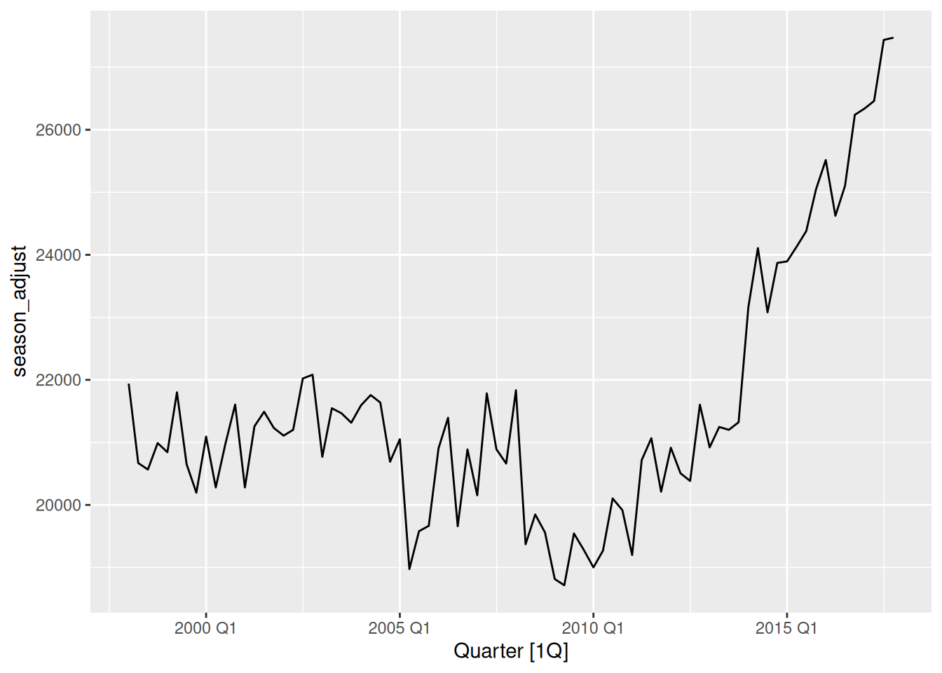

Forecast the next two years of the series using an additive damped trend method applied to the seasonally adjusted data. (This can be specified using decomposition_model().)

stletsdamped <- decomposition_model(
  STL(Trips),
  ETS(season_adjust ~ error("A") + trend("Ad") + season("N"))
)
aus_trips |>
  model(dcmp_AAdN = stletsdamped) |>
  forecast(h = "2 years") |>
  autoplot(aus_trips)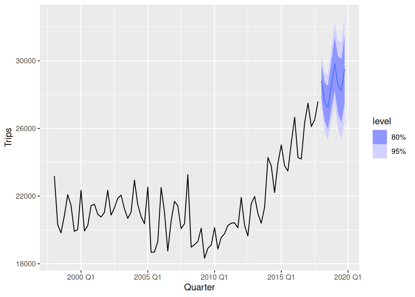

Forecast the next two years of the series using an appropriate model for Holt’s linear method applied to the seasonally adjusted data (as before but without damped trend).

stletstrend <- decomposition_model(
  STL(Trips),
  ETS(season_adjust ~ error("A") + trend("A") + season("N"))
)
aus_trips |>
  model(dcmp_AAN = stletstrend) |>
  forecast(h = "2 years") |>
  autoplot(aus_trips)

Now use ETS() to choose a seasonal model for the data.

fit <- aus_trips |>
        model(ets = ETS(Trips))

fit |> report()

Series: Trips 
Model: ETS(A,A,A) 
  Smoothing parameters:
    alpha = 0.4495675 
    beta  = 0.04450178 
    gamma = 0.0001000075 

  Initial states:
     l[0]      b[0]      s[0]     s[-1]     s[-2]    s[-3]
 21689.64 -58.46946 -125.8548 -816.3416 -324.5553 1266.752

  sigma^2:  699901.4

     AIC     AICc      BIC 
1436.829 1439.400 1458.267

fit |> tidy()

# A tibble: 9 × 3
  .model term      estimate
  <chr>  <chr>        <dbl>
1 ets    alpha     0.450   
2 ets    beta      0.0445  
3 ets    gamma     0.000100
4 ets    l[0]  21690.      
5 ets    b[0]    -58.5     
6 ets    s[0]   -126.      
7 ets    s[-1]  -816.      
8 ets    s[-2]  -325.      
9 ets    s[-3]  1267.

fit |> forecast(h = "2 years") |>
  autoplot(aus_trips)

Compare the RMSE of the ETS model with the RMSE of the models you obtained using STL decompositions. Which gives the better in-sample fits?

fit <- aus_trips |>
  model(
    dcmp_AAdN = stletsdamped,
    dcmp_AAN = stletstrend,
    ets = ETS(Trips)
  )

fit |>
    select(ets) |>
    tidy()

# A tibble: 9 × 3
  .model term      estimate
  <chr>  <chr>        <dbl>
1 ets    alpha     0.450   
2 ets    beta      0.0445  
3 ets    gamma     0.000100
4 ets    l[0]  21690.      
5 ets    b[0]    -58.5     
6 ets    s[0]   -126.      
7 ets    s[-1]  -816.      
8 ets    s[-2]  -325.      
9 ets    s[-3]  1267.

fit |>
    select(ets) |>
    report()

Series: Trips 
Model: ETS(A,A,A) 
  Smoothing parameters:
    alpha = 0.4495675 
    beta  = 0.04450178 
    gamma = 0.0001000075 

  Initial states:
     l[0]      b[0]      s[0]     s[-1]     s[-2]    s[-3]
 21689.64 -58.46946 -125.8548 -816.3416 -324.5553 1266.752

  sigma^2:  699901.4

     AIC     AICc      BIC 
1436.829 1439.400 1458.267

accuracy(fit)

# A tibble: 3 × 10
  .model    .type       ME  RMSE   MAE   MPE  MAPE  MASE RMSSE     ACF1
  <chr>     <chr>    <dbl> <dbl> <dbl> <dbl> <dbl> <dbl> <dbl>    <dbl>
1 dcmp_AAdN Training 103.   763.  576. 0.367  2.72 0.607 0.629 -0.0174 
2 dcmp_AAN  Training  99.7  763.  574. 0.359  2.71 0.604 0.628 -0.0182 
3 ets       Training 105.   794.  604. 0.379  2.86 0.636 0.653 -0.00151

The STL decomposition forecasts using the additive trend model, ETS(A,A,N), is slightly better in-sample.
However, note that this is a biased comparison as the models have different numbers of parameters.

Compare the forecasts from the three approaches? Which seems most reasonable?

fit |>
  forecast(h = "2 years") |>
  autoplot(aus_trips, level = NULL)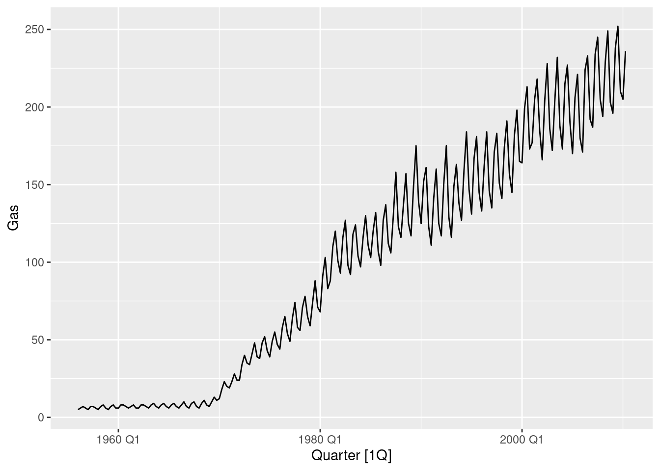

The forecasts are almost identical. So I’ll use the decomposition model with additive trend as it has the smallest RMSE.

Check the residuals of your preferred model.

best <- fit |>
  select(dcmp_AAN)

report(best)

Series: Trips 
Model: STL decomposition model 
Combination: season_adjust + season_year

========================================

Series: season_adjust 
Model: ETS(A,A,N) 
  Smoothing parameters:
    alpha = 0.4806411 
    beta  = 0.04529462 

  Initial states:
     l[0]     b[0]
 21366.07 1.279692

  sigma^2:  585061

     AIC     AICc      BIC 
1418.816 1419.627 1430.727 

Series: season_year 
Model: SNAIVE 

sigma^2: 3210.8552

augment(best) |> gg_tsdisplay(.resid, lag_max = 24, plot_type = "histogram")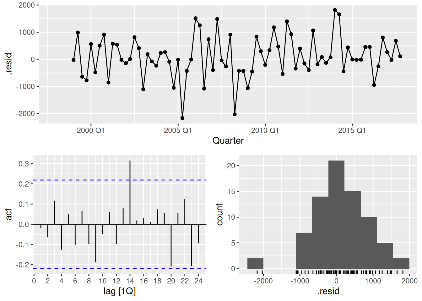

augment(best) |> features(.innov, ljung_box, lag = 24)

# A tibble: 1 × 3
  .model   lb_stat lb_pvalue
  <chr>      <dbl>     <dbl>
1 dcmp_AAN    33.3    0.0976

The residuals look okay however there still remains some significant auto-correlation. Nevertheless, the results pass the Ljung-Box test.
The large spike at lag 14 can probably be ignored.

fpp3 8.8, Ex11

For this exercise use the quarterly number of arrivals to Australia from New Zealand, 1981 Q1 – 2012 Q3, from data set aus_arrivals.

Make a time plot of your data and describe the main features of the series.

nzarrivals <- aus_arrivals |> filter(Origin == "NZ")
nzarrivals |> autoplot(Arrivals / 1e3) + labs(y = "Thousands of people")

The data has an upward trend.
The data has a seasonal pattern which increases in size approximately proportionally to the average number of people who arrive per year. Therefore, the data has multiplicative seasonality.

Create a training set that withholds the last two years of available data. Forecast the test set using an appropriate model for Holt-Winters’ multiplicative method.

nz_tr <- nzarrivals |>
  slice(1:(n() - 8))
nz_tr |>
  model(ETS(Arrivals ~ error("M") + trend("A") + season("M"))) |>
  forecast(h = "2 years") |>
  autoplot() +
  autolayer(nzarrivals, Arrivals)

Why is multiplicative seasonality necessary here?

The multiplicative seasonality is important in this example because the seasonal pattern increases in size proportionally to the level of the series.
The behaviour of the seasonal pattern will be captured and projected in a model with multiplicative seasonality.

Forecast the two-year test set using each of the following methods:

an ETS model;

an additive ETS model applied to a log transformed series;

a seasonal naïve method;

an STL decomposition applied to the log transformed data followed by an ETS model applied to the seasonally adjusted (transformed) data.

fc <- nz_tr |>
  model(
    ets = ETS(Arrivals),
    log_ets = ETS(log(Arrivals)),
    snaive = SNAIVE(Arrivals),
    stl = decomposition_model(STL(log(Arrivals)), ETS(season_adjust))
  ) |>
  forecast(h = "2 years")

fc |>
  autoplot(level = NULL) +
  autolayer(filter(nzarrivals, year(Quarter) > 2000), Arrivals)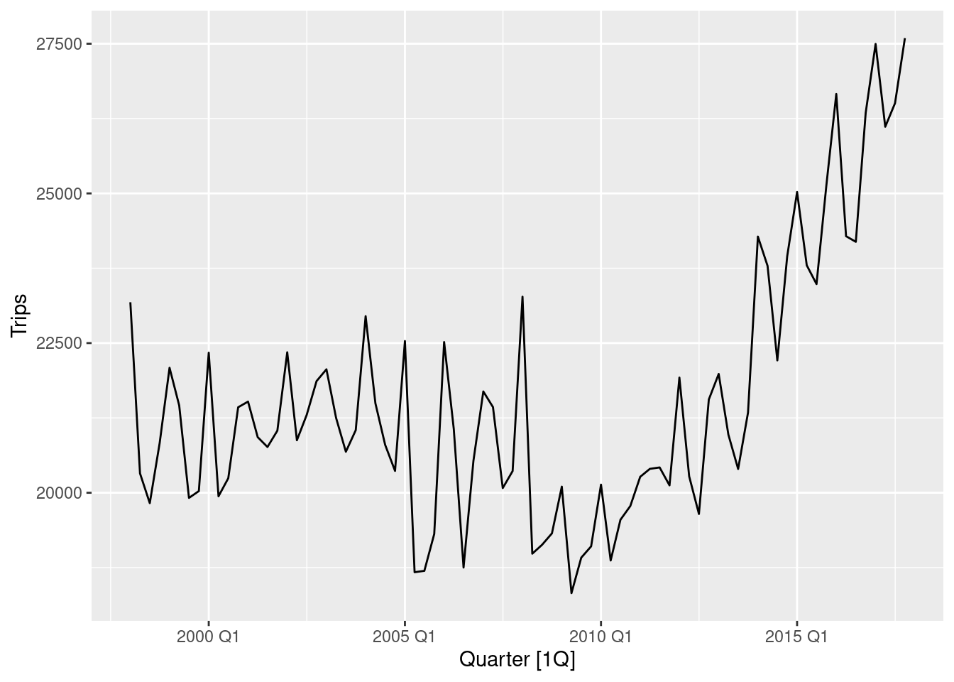

fc |>
  autoplot(level = NULL) +
  autolayer(nzarrivals, Arrivals)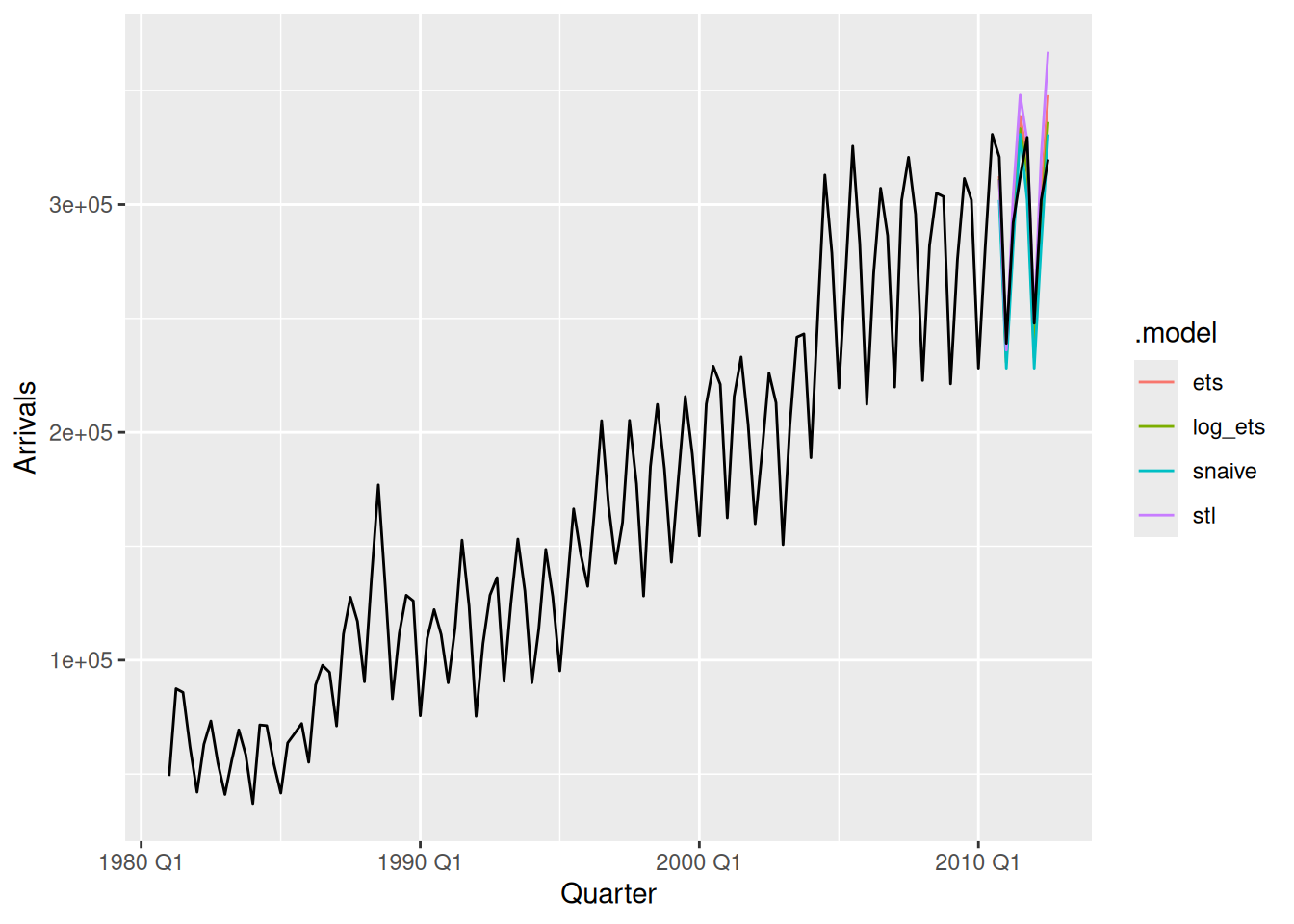

Which method gives the best forecasts? Does it pass the residual tests?

fc |>
  accuracy(nzarrivals)

# A tibble: 4 × 11
  .model  Origin .type      ME   RMSE    MAE    MPE  MAPE  MASE RMSSE    ACF1
  <chr>   <chr>  <chr>   <dbl>  <dbl>  <dbl>  <dbl> <dbl> <dbl> <dbl>   <dbl>
1 ets     NZ     Test   -3495. 14913. 11421. -0.964  3.78 0.768 0.771 -0.0260
2 log_ets NZ     Test    2467. 13342. 11904.  1.03   4.03 0.800 0.689 -0.0786
3 snaive  NZ     Test    9709. 18051. 17156.  3.44   5.80 1.15  0.933 -0.239 
4 stl     NZ     Test  -12535. 22723. 16172. -4.02   5.23 1.09  1.17   0.109

The best method is the ETS model on the logged data (based on RMSE), and it passes the residuals tests.

log_ets <- nz_tr |>
  model(ETS(log(Arrivals)))
log_ets |> gg_tsresiduals()

augment(log_ets) |>
  features(.innov, ljung_box, lag = 12)

# A tibble: 1 × 4
  Origin .model             lb_stat lb_pvalue
  <chr>  <chr>                <dbl>     <dbl>
1 NZ     ETS(log(Arrivals))    11.0     0.530

Compare the same four methods using time series cross-validation instead of using a training and test set. Do you come to the same conclusions?

nz_cv <- nzarrivals |>
  slice(1:(n() - 3)) |>
  stretch_tsibble(.init = 36, .step = 3)

nz_cv |>
  model(
    ets = ETS(Arrivals),
    log_ets = ETS(log(Arrivals)),
    snaive = SNAIVE(Arrivals),
    stl = decomposition_model(STL(log(Arrivals)), ETS(season_adjust))
  ) |>
  forecast(h = 3) |>
  accuracy(nzarrivals)

# A tibble: 4 × 11
  .model  Origin .type    ME   RMSE    MAE   MPE  MAPE  MASE RMSSE  ACF1
  <chr>   <chr>  <chr> <dbl>  <dbl>  <dbl> <dbl> <dbl> <dbl> <dbl> <dbl>
1 ets     NZ     Test  4627. 15327. 11799.  2.23  6.45 0.793 0.797 0.283
2 log_ets NZ     Test  4388. 15047. 11566.  1.99  6.36 0.778 0.782 0.268
3 snaive  NZ     Test  8244. 18768. 14422.  3.83  7.76 0.970 0.976 0.566
4 stl     NZ     Test  4252. 15618. 11873.  2.04  6.25 0.798 0.812 0.244

An initial fold size (.init) of 36 has been selected to ensure that sufficient data is available to make reasonable forecasts.
A step size of 3 (and forecast horizon of 3) has been used to reduce the computation time.
The ETS model on the log data still appears best (based on 3-step ahead forecast RMSE).

fpp3 8.8, Ex12

Apply cross-validation techniques to produce 1 year ahead ETS and seasonal naïve forecasts for Portland cement production (from aus_production). Use a stretching data window with initial size of 5 years, and increment the window by one observation.

cement_cv <- aus_production |>
  slice(1:(n() - 4)) |>
  stretch_tsibble(.init = 5 * 4)

fc <- cement_cv |>
  model(ETS(Cement), SNAIVE(Cement)) |>
  forecast(h = "1 year")

Compute the MSE of the resulting 4-step-ahead errors. Comment on which forecasts are more accurate. Is this what you expected?

fc |>
  group_by(.id, .model) |>
  mutate(h = row_number()) |>
  ungroup() |>
  as_fable(response = "Cement", distribution = Cement) |>
  accuracy(aus_production, by = c(".model", "h"))

# A tibble: 8 × 11
  .model           h .type      ME  RMSE   MAE    MPE  MAPE  MASE RMSSE     ACF1
  <chr>        <int> <chr>   <dbl> <dbl> <dbl>  <dbl> <dbl> <dbl> <dbl>    <dbl>
1 ETS(Cement)      1 Test  -0.0902  82.9  60.1 -0.227  3.95 0.597 0.625 -0.00185
2 ETS(Cement)      2 Test  -0.653  101.   72.0 -0.325  4.74 0.708 0.756  0.495  
3 ETS(Cement)      3 Test  -1.71   119.   87.0 -0.492  5.80 0.856 0.894  0.616  
4 ETS(Cement)      4 Test  -0.729  137.  102.  -0.543  6.65 1.01  1.03   0.699  
5 SNAIVE(Ceme…     1 Test  30.9    138.  107.   1.97   6.99 1.06  1.04   0.640  
6 SNAIVE(Ceme…     2 Test  30.0    139.  107.   1.90   6.96 1.05  1.04   0.649  
7 SNAIVE(Ceme…     3 Test  29.5    139.  107.   1.85   6.95 1.05  1.04   0.651  
8 SNAIVE(Ceme…     4 Test  30.8    140.  108    1.91   6.99 1.06  1.05   0.637

The ETS results are better for all horizons, although getting closer as h increases. With a long series like this, I would expect ETS to do better as it should have no trouble estimating the parameters, and it will include trends if required.

fpp3 8.8, Ex13

Compare ETS(), SNAIVE() and decomposition_model(STL, ???) on the following five time series. You might need to use a Box-Cox transformation for the STL decomposition forecasts. Use a test set of three years to decide what gives the best forecasts.

Beer production from aus_production

fc <- aus_production |>
  filter(Quarter < max(Quarter - 11)) |>
  model(
    ETS(Beer),
    SNAIVE(Beer),
    stlm = decomposition_model(STL(log(Beer)), ETS(season_adjust))
  ) |>
  forecast(h = "3 years")
fc |>
  autoplot(filter_index(aus_production, "2000 Q1" ~ .), level = NULL)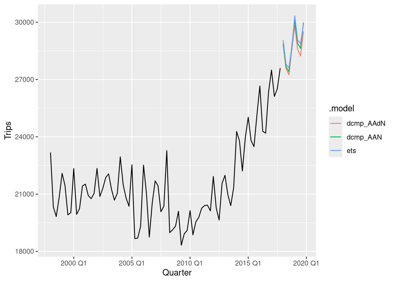

fc |> accuracy(aus_production)

# A tibble: 3 × 10
  .model       .type     ME  RMSE   MAE      MPE  MAPE  MASE RMSSE  ACF1
  <chr>        <chr>  <dbl> <dbl> <dbl>    <dbl> <dbl> <dbl> <dbl> <dbl>
1 ETS(Beer)    Test   0.127  9.62  8.92  0.00998  2.13 0.563 0.489 0.376
2 SNAIVE(Beer) Test  -2.92  10.8   9.75 -0.651    2.34 0.616 0.549 0.325
3 stlm         Test  -2.85   9.87  8.95 -0.719    2.16 0.565 0.502 0.283

ETS and STLM do best for this dataset based on the test set performance.

Bricks production from aus_production

tidy_bricks <- aus_production |>
  filter(!is.na(Bricks))
fc <- tidy_bricks |>
  filter(Quarter < max(Quarter - 11)) |>
  model(
    ets = ETS(Bricks),
    snaive = SNAIVE(Bricks),
    STLM = decomposition_model(STL(log(Bricks)), ETS(season_adjust))
  ) |>
  forecast(h = "3 years")
fc |> autoplot(filter_index(aus_production, "1980 Q1" ~ .), level = NULL)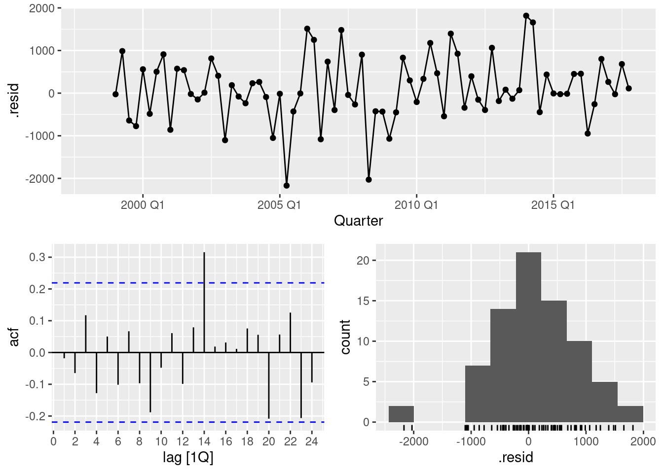

fc |> accuracy(tidy_bricks)

# A tibble: 3 × 10
  .model .type    ME  RMSE   MAE   MPE  MAPE  MASE RMSSE    ACF1
  <chr>  <chr> <dbl> <dbl> <dbl> <dbl> <dbl> <dbl> <dbl>   <dbl>
1 STLM   Test   9.71  18.7  14.9 2.29   3.65 0.411 0.378  0.0933
2 ets    Test   2.27  17.5  13.2 0.474  3.31 0.365 0.354  0.339 
3 snaive Test  32.6   36.5  32.6 7.85   7.85 0.898 0.739 -0.322

ETS and STLM do best for this dataset based on the test set performance.

Cost of drug subsidies for diabetes (ATC2 == "A10") and corticosteroids (ATC2 == "H02") from PBS

subsidies <- PBS |>
  filter(ATC2 %in% c("A10", "H02")) |>
  group_by(ATC2) |>
  summarise(Cost = sum(Cost))
subsidies |>
  autoplot(vars(Cost)) +
  facet_grid(vars(ATC2), scales = "free_y")

fc <- subsidies |>
  filter(Month < max(Month) - 35) |>
  model(
    ETS(Cost),
    SNAIVE(Cost),
    STLM = decomposition_model(STL(log(Cost)), ETS(season_adjust))) |>
  forecast(h = "3 years")
fc |> autoplot(subsidies, level = NULL)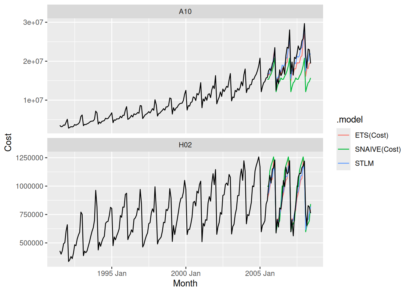

fc |>
  accuracy(subsidies) |>
  arrange(ATC2)

# A tibble: 6 × 11
  .model      ATC2  .type      ME   RMSE    MAE    MPE  MAPE  MASE RMSSE    ACF1
  <chr>       <chr> <chr>   <dbl>  <dbl>  <dbl>  <dbl> <dbl> <dbl> <dbl>   <dbl>
1 ETS(Cost)   A10   Test   1.38e6 2.36e6 1.85e6  5.83   8.74 1.89  2.00   0.177 
2 SNAIVE(Cos… A10   Test   4.32e6 5.18e6 4.33e6 19.8   19.9  4.42  4.40   0.638 
3 STLM        A10   Test   3.27e5 1.62e6 1.32e6  0.783  6.73 1.35  1.37  -0.0894
4 ETS(Cost)   H02   Test   2.70e4 7.65e4 6.45e4  1.99   7.05 1.09  1.07  -0.0990
5 SNAIVE(Cos… H02   Test  -1.48e4 8.55e4 7.16e4 -1.31   7.88 1.21  1.20   0.0226
6 STLM        H02   Test   2.24e4 6.83e4 5.63e4  1.61   6.24 0.951 0.959 -0.217

The STLM method appears to perform best for both series.

Total food retailing turnover for Australia from aus_retail.

food_retail <- aus_retail |>
  filter(Industry == "Food retailing") |>
  summarise(Turnover = sum(Turnover))

fc <- food_retail |>
  filter(Month < max(Month) - 35) |>
  model(
    ETS(Turnover),
    SNAIVE(Turnover),
    STLM = decomposition_model(STL(log(Turnover)), ETS(season_adjust))
  ) |>
  forecast(h = "3 years")
fc |>
  autoplot(filter_index(food_retail, "2005 Jan" ~ .), level = NULL)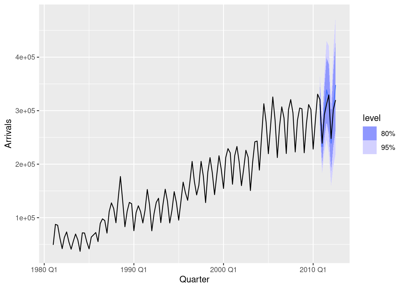

fc |> accuracy(food_retail)

# A tibble: 3 × 10
  .model           .type     ME  RMSE   MAE    MPE  MAPE  MASE RMSSE  ACF1
  <chr>            <chr>  <dbl> <dbl> <dbl>  <dbl> <dbl> <dbl> <dbl> <dbl>
1 ETS(Turnover)    Test  -151.   194.  170. -1.47   1.65 0.639 0.634 0.109
2 SNAIVE(Turnover) Test   625.   699.  625.  5.86   5.86 2.35  2.29  0.736
3 STLM             Test   -12.8  170.  144. -0.189  1.36 0.543 0.554 0.314

The STLM model does better than other approaches for this dataset.

fpp3 8.8, Ex14

Use ETS() to select an appropriate model for the following series: total number of trips across Australia using tourism, the closing prices for the four stocks in gafa_stock, and the lynx series in pelt. Does it always give good forecasts?

tourism

aus_trips <- tourism |>
  summarise(Trips = sum(Trips))
aus_trips |>
  model(ETS(Trips)) |>
  report()

Series: Trips 
Model: ETS(A,A,A) 
  Smoothing parameters:
    alpha = 0.4495675 
    beta  = 0.04450178 
    gamma = 0.0001000075 

  Initial states:
     l[0]      b[0]      s[0]     s[-1]     s[-2]    s[-3]
 21689.64 -58.46946 -125.8548 -816.3416 -324.5553 1266.752

  sigma^2:  699901.4

     AIC     AICc      BIC 
1436.829 1439.400 1458.267

aus_trips |>
  model(ETS(Trips)) |>
  forecast() |>
  autoplot(aus_trips)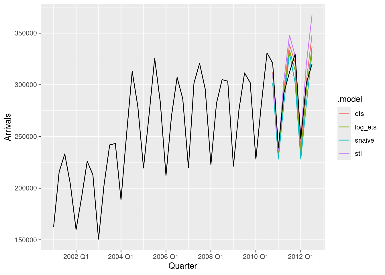

Forecasts appear reasonable.

GAFA stock

gafa_regular <- gafa_stock |>
  group_by(Symbol) |>
  mutate(trading_day = row_number()) |>
  ungroup() |>
  as_tsibble(index = trading_day, regular = TRUE)

gafa_stock |> autoplot(Close)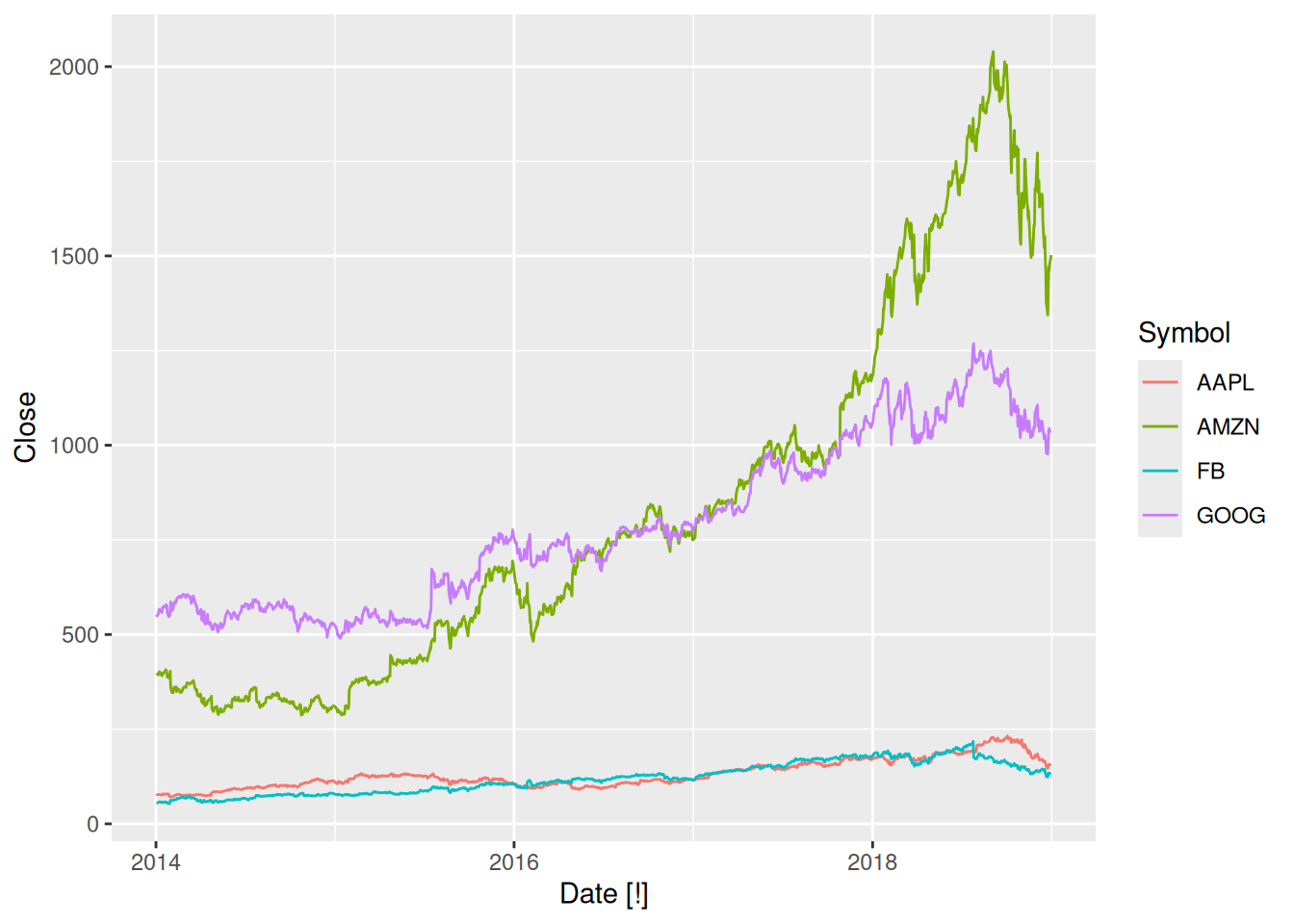

gafa_regular |>
  model(ETS(Close))

# A mable: 4 x 2
# Key:     Symbol [4]
  Symbol `ETS(Close)`
  <chr>       <model>
1 AAPL   <ETS(M,N,N)>
2 AMZN   <ETS(M,N,N)>
3 FB     <ETS(M,N,N)>
4 GOOG   <ETS(M,N,N)>

gafa_regular |>
  model(ETS(Close)) |>
  forecast(h = 50) |>
  autoplot(gafa_regular |> group_by_key() |> slice((n() - 100):n()))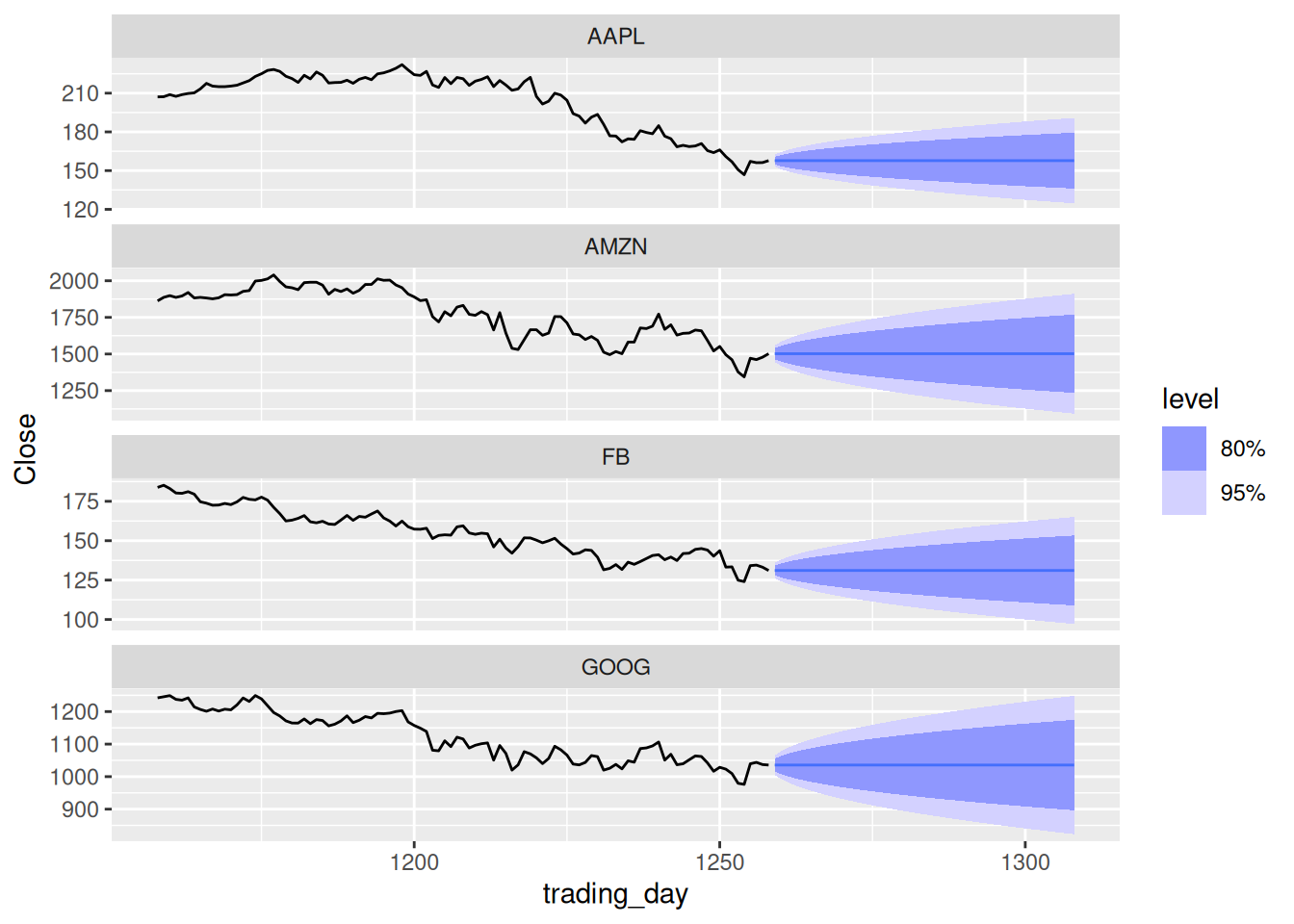

Forecasts look reasonable for an efficient market.

Pelt trading records

pelt |>
  model(ETS(Lynx))

# A mable: 1 x 1
   `ETS(Lynx)`
       <model>
1 <ETS(A,N,N)>

pelt |>
  model(ETS(Lynx)) |>
  forecast(h = 10) |>
  autoplot(pelt)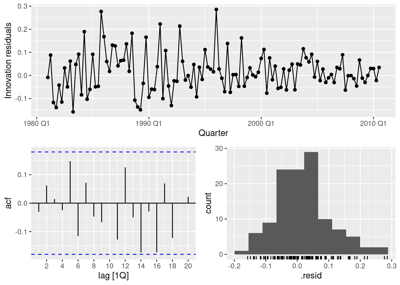

Here the cyclic behaviour of the lynx data is completely lost.
ETS models are not designed to handle cyclic data, so there is nothing that can be done to improve this.

Find an example where it does not work well. Can you figure out why?

ETS does not work well on cyclic data, as seen in the pelt dataset above.

fpp3 8.8, Ex15

Show that the point forecasts from an ETS(M,A,M) model are the same as those obtained using Holt-Winters’ multiplicative method.

Point forecasts from the multiplicative Holt-Winters’ method: \hat{y}_{t+h|t} = (\ell_t + hb_t)s_{t+ h - m(k+1)} where k is the integer part of (h-1)/m.

An ETS(M,A,M) model is given by \begin{align*} y_t & = (\ell_{t-1}+b_{t-1})s_{t-m}(1+\varepsilon_t) \\ \ell_t & = (\ell_{t-1}+b_{t-1})(1+\alpha\varepsilon_t) \\ b_t & = b_{t-1} + \beta(\ell_{t-1}+b_{t-1})\varepsilon_t \\ s_t & = s_{t-m} (1+\gamma\varepsilon_t) \end{align*} So y_{T+h} is given by y_{T+h} = (\ell_{T+h-1}+b_{T+h-1})s_{T+h-m}(1+\varepsilon_{T+h-m}) Replacing \varepsilon_{t} by zero for t>T, and substituting in from the above equations, we obtain \hat{y}_{T+h} = (\ell_{T+h-2}+2b_{T+h-2})s_{T+h-m} Repeating the process a few times leads to \hat{y}_{T+h} = (\ell_{T}+hb_{T})s_{T+h-m}

Now if h \le m, then we know the value of s_{T+h-m}.

If m < h \le 2m, then we can write s_{T+h-m} = s_{T+h-2m} (1 + \gamma\varepsilon_{T+h-m}) and replace \varepsilon_{T+h-m} by 0

If 2m < h \le 3m, then we can write s_{T+h-m} = s_{T+h-3m} (1 + \gamma\varepsilon_{T+h-m})(1+\gamma\varepsilon_{T+h-2m}) and replace both \varepsilon_{T+h-m} and \varepsilon_{T+h-2m} by 0

etc.

So we can replace s_{T+h-m} by s_{T+h - m(k+1)} where k is the integer part of (k-1)/m.

Thus \hat{y}_{T+h|T} = (\ell_{T}+hb_{T})s_{T+h -m(k+1)} as required.