Exercise Week 6: Solutions

library(fpp3)

fpp3 8.8, Ex1

Consider the the number of pigs slaughtered in Victoria, available in the aus_livestock dataset.

Use the ETS() function in R to estimate the equivalent model for simple exponential smoothing. Find the optimal values of \alpha and \ell_0, and generate forecasts for the next four months.

fit <- aus_livestock |>
  filter(Animal == "Pigs", State == "Victoria") |>
  model(ses = ETS(Count ~ error("A") + trend("N") + season("N")))
report(fit)

Series: Count 
Model: ETS(A,N,N) 
  Smoothing parameters:
    alpha = 0.3221247 

  Initial states:
     l[0]
 100646.6

  sigma^2:  87480760

     AIC     AICc      BIC 
13737.10 13737.14 13750.07

Optimal values are \alpha = 0.3221247 and \ell_0 = 100646.6

fc <- fit |> forecast(h = "4 months")
fc

# A fable: 4 x 6 [1M]
# Key:     Animal, State, .model [1]
  Animal State    .model    Month
  <fct>  <fct>    <chr>     <mth>
1 Pigs   Victoria ses    2019 Jan
2 Pigs   Victoria ses    2019 Feb
3 Pigs   Victoria ses    2019 Mar
4 Pigs   Victoria ses    2019 Apr
# ℹ 2 more variables: Count <dist>, .mean <dbl>

fc |>
  autoplot(filter(aus_livestock, Month >= yearmonth("2010 Jan")))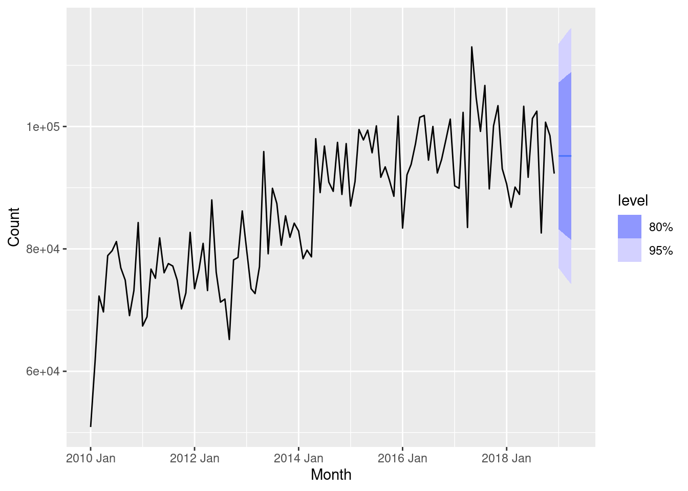

Compute a 95% prediction interval for the first forecast using \hat{y} \pm 1.96s where s is the standard deviation of the residuals. Compare your interval with the interval produced by R.

s <- augment(fit) |>
  pull(.resid) |>
  sd()
yhat <- fc |>
  pull(.mean) |>
  head(1)
yhat + c(-1, 1) * 1.96 * s

[1]  76871.01 113502.10

fc |>
  head(1) |>
  mutate(interval = hilo(Count, 95)) |>
  pull(interval)

<hilo[1]>
[1] [76854.79, 113518.3]95

The intervals are close but not identical. This is because R estimates the variance of the residuals differently, taking account of the degrees of freedom properly (and also using a more accurate critical value rather than just 1.96).

Try the following.

res <- augment(fit) |> pull(.resid)
s <- sqrt(sum(res^2) / (length(res) - NROW(tidy(fit))))
yhat + c(-1, 1) * qnorm(0.975) * s

[1]  76854.79 113518.33

fpp3 8.8, Ex2

Write your own function to implement simple exponential smoothing. The function should take arguments y (the response data), alpha (the smoothing parameter \alpha) and level (the initial level \ell_0). It should return the forecast of the next observation in the series. Does it give the same forecast as ETS()?

my_ses <- function(y, alpha, level) {
  yhat <- numeric(length(y) + 1)
  yhat[1] <- level
  for (i in 2:(length(yhat))) {
    yhat[i] <- alpha * y[i - 1] + (1 - alpha) * yhat[i - 1]
  }
  return(last(yhat))
}

vic_pigs_vec <- aus_livestock |>
  filter(Animal == "Pigs", State == "Victoria") |>
  pull(Count)

ses_fc <- vic_pigs_vec |>
  my_ses(alpha = 0.3221, level = 100646.6)

c(my_ses = ses_fc, fable = fc$.mean[1])

  my_ses    fable 
95186.59 95186.56

Yes, the same forecasts are obtained. The slight differences are due to rounding of \alpha and \ell_0.

fpp3 8.8, Ex3

Modify your function from the previous exercise to return the sum of squared errors rather than the forecast of the next observation. Then use the optim() function to find the optimal values of \alpha and \ell_0. Do you get the same values as the ETS() function?

my_ses_sse <- function(par, y) {
  alpha <- par[1]
  level <- par[2]
  n <- length(y)
  yhat <- numeric(n)
  yhat[1] <- level
  for (i in 2:n) {
    yhat[i] <- alpha * y[i - 1] + (1 - alpha) * yhat[i - 1]
  }
  return(sum((y - yhat)^2))
}

optim(c(0.1, vic_pigs_vec[1]), my_ses_sse, y = vic_pigs_vec)$par

[1] 3.220344e-01 1.005254e+05

tidy(fit)

# A tibble: 2 × 5
  Animal State    .model term    estimate
  <fct>  <fct>    <chr>  <chr>      <dbl>
1 Pigs   Victoria ses    alpha      0.322
2 Pigs   Victoria ses    l[0]  100647.

Similar, but not identical estimates. This is due to different starting values being used.

fpp3 8.8, Ex4

Combine your previous two functions to produce a function that both finds the optimal values of \alpha and \ell_0, and produces a forecast of the next observation in the series.

my_ses <- function(y) {
  par <- optim(c(0.1, y[1]), my_ses_sse, y = y)$par
  alpha <- par[1]
  level <- par[2]
  yhat <- numeric(length(y) + 1)
  yhat[1] <- level
  for (i in 2:(length(yhat))) {
    yhat[i] <- alpha * y[i - 1] + (1 - alpha) * yhat[i - 1]
  }
  return(last(yhat))
}
my_ses(vic_pigs_vec)

[1] 95186.69

fpp3 8.8, Ex5

Data set global_economy contains the annual Exports from many countries. Select one country to analyse.

Plot the Exports series and discuss the main features of the data.

global_economy |>
  filter(Country == "Argentina") |>
  autoplot(Exports)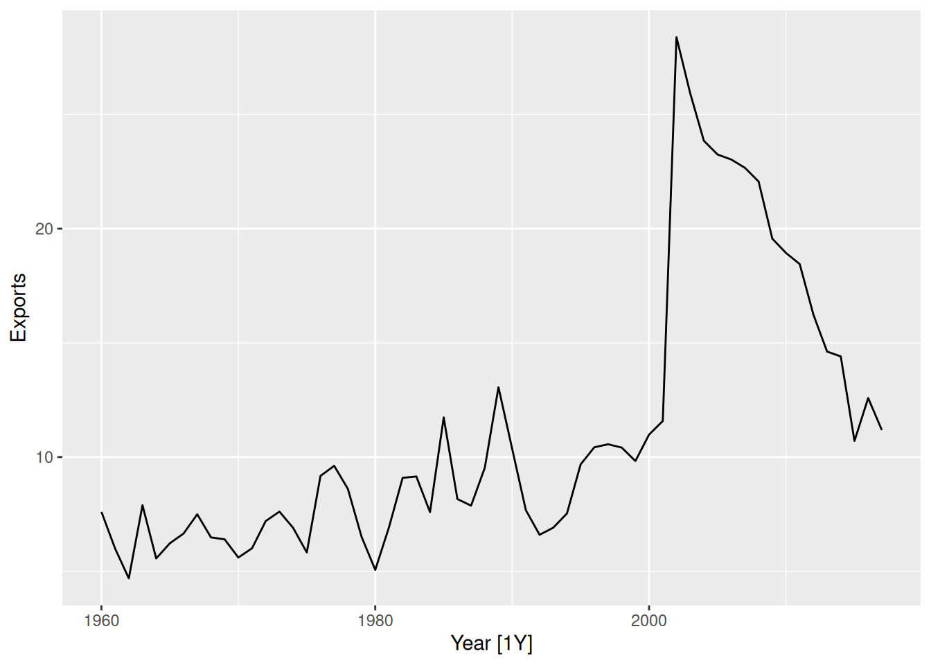

There is a huge jump in Exports in 2002, due to the deregulation of the Argentinian peso. Since then, Exports (as a percentage of GDP) has gradually returned to 1990 levels.

Use an ETS(A,N,N) model to forecast the series, and plot the forecasts.

etsANN <- global_economy |>
  filter(Country == "Argentina") |>
  model(ETS(Exports ~ error("A") + trend("N") + season("N")))
etsANN |>
  forecast(h = 10) |>
  autoplot(global_economy)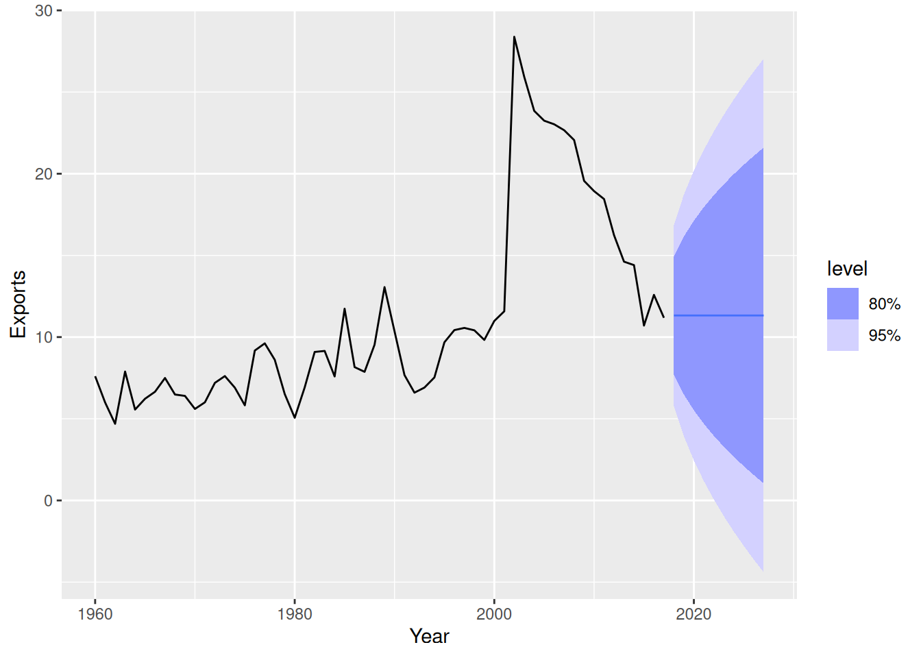

Compute the RMSE values for the training data.

accuracy(etsANN) |> select(RMSE)

# A tibble: 1 × 1
   RMSE
  <dbl>
1  2.78

Compare the results to those from an ETS(A,A,N) model. (Remember that the trended model is using one more parameter than the simpler model.) Discuss the merits of the two forecasting methods for this data set.

fit <- global_economy |>
  filter(Country == "Argentina") |>
  model(
    ses = ETS(Exports ~ error("A") + trend("N") + season("N")),
    holt = ETS(Exports ~ error("A") + trend("A") + season("N"))
  )
accuracy(fit)

# A tibble: 2 × 11
  Country   .model .type         ME  RMSE   MAE   MPE  MAPE  MASE RMSSE    ACF1
  <fct>     <chr>  <chr>      <dbl> <dbl> <dbl> <dbl> <dbl> <dbl> <dbl>   <dbl>
1 Argentina ses    Training 0.0762   2.78  1.62 -1.73  15.7 0.983 0.986 0.00902
2 Argentina holt   Training 0.00795  2.78  1.64 -2.51  15.9 0.994 0.986 0.0271

There is very little difference in training RMSE between these models. So the extra parameter is not doing much.

Compare the forecasts from both methods. Which do you think is best?

fit |>
  forecast(h = 10) |>
  autoplot(global_economy)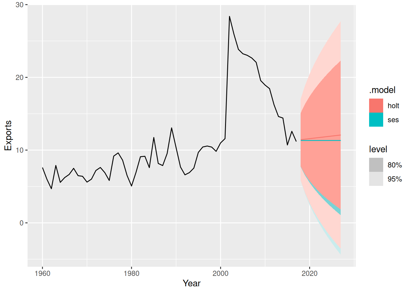

The forecasts are similar. In this case, the simpler model is preferred.

Calculate a 95% prediction interval for the first forecast for each series, using the RMSE values and assuming normal errors. Compare your intervals with those produced using R.

standard error. (from RMSE)
mean (from forecast)

s <- accuracy(fit) |> pull(RMSE)
yhat <- forecast(fit, h = 1) |> pull(.mean)
# SES
yhat[1] + c(-1, 1) * qnorm(0.975) * s[1]

[1]  5.882074 16.764136

# Holt
yhat[2] + c(-1, 1) * qnorm(0.975) * s[2]

[1]  5.989515 16.872908

fit |>
  forecast(h = 1) |>
  mutate(PI = hilo(Exports, level = 95))

# A fable: 2 x 6 [1Y]
# Key:     Country, .model [2]
  Country   .model  Year
  <fct>     <chr>  <dbl>
1 Argentina ses     2018
2 Argentina holt    2018
# ℹ 3 more variables: Exports <dist>, .mean <dbl>, PI <hilo>

Using RMSE yields narrower prediction interval while using the values from hilo() function gives wider prediction interval.
Using RMSE has failed to take account of the degrees of freedom for each model. Compare the following

sse <- augment(fit) |>
  as_tibble() |>
  group_by(.model) |>
  summarise(s = sum(.resid^2)) |>
  pull(s)

n <- global_economy |>
  filter(Country == "Argentina") |>
    nrow()

# sse method= alpha, level=> 2
# holt linear = alpha, level, trend, b => 4

s <- sqrt(sse / (n - c(2, 4)))

# SES
yhat[1] + c(-1, 1) * qnorm(0.975) * s[1]

[1]  5.785088 16.861122

# Holt
yhat[2] + c(-1, 1) * qnorm(0.975) * s[2]

[1]  5.79226 17.07016

fpp3 8.8, Ex6

Forecast the Chinese GDP from the global_economy data set using an ETS model. Experiment with the various options in the ETS() function to see how much the forecasts change with damped trend, or with a Box-Cox transformation. Try to develop an intuition of what each is doing to the forecasts.

[Hint: use h=20 when forecasting, so you can clearly see the differences between the various options when plotting the forecasts.]

china <- global_economy |>
  filter(Country == "China")
china |> autoplot(GDP)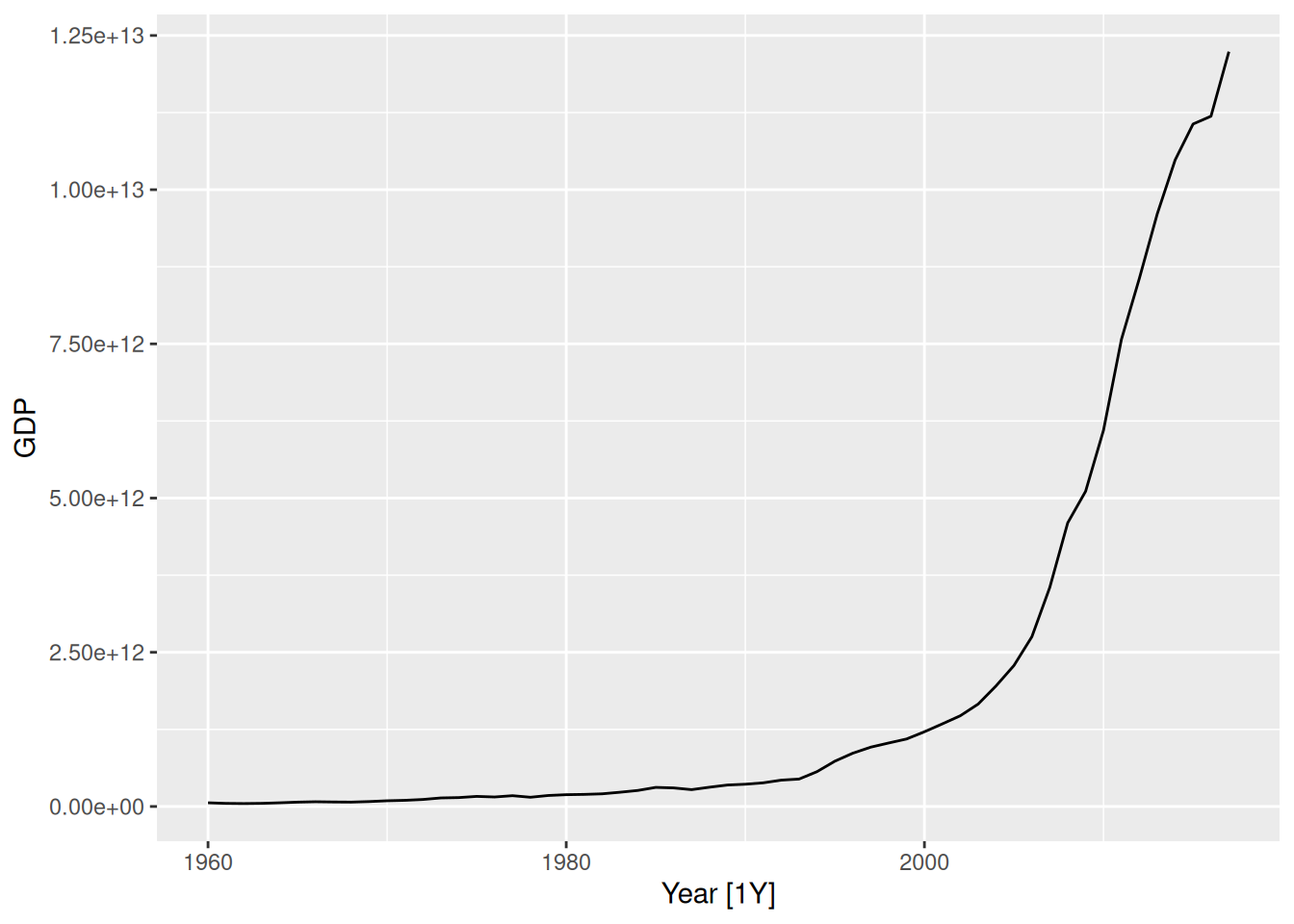

It clearly needs a relatively strong transformation due to the increasing variance.

china |> autoplot(box_cox(GDP, 0.2))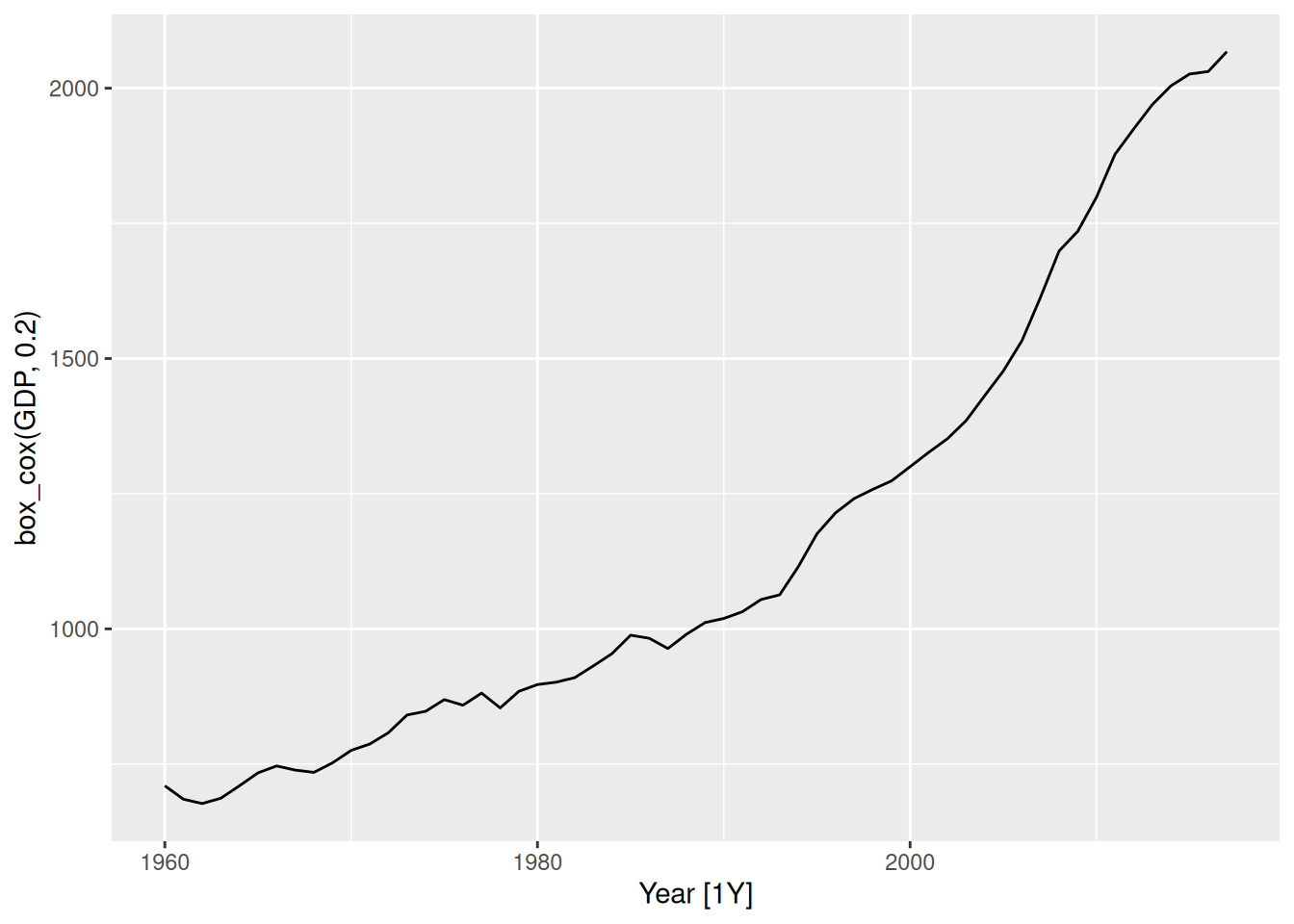

china |> features(GDP, guerrero)

# A tibble: 1 × 2
  Country lambda_guerrero
  <fct>             <dbl>
1 China           -0.0345

Making \lambda=0.2 looks ok.
The Guerrero method suggests an even stronger transformation. Let’s also try a log.

fit <- china |>
  model(
    ets = ETS(GDP),
    ets_damped = ETS(GDP ~ trend("Ad")),
    ets_bc = ETS(box_cox(GDP, 0.2)),
    ets_log = ETS(log(GDP))
  )

fit

# A mable: 1 x 5
# Key:     Country [1]
  Country          ets    ets_damped       ets_bc      ets_log
  <fct>        <model>       <model>      <model>      <model>
1 China   <ETS(M,A,N)> <ETS(M,Ad,N)> <ETS(A,A,N)> <ETS(A,A,N)>

augment(fit)

# A tsibble: 232 x 7 [1Y]
# Key:       Country, .model [4]
   Country .model  Year          GDP      .fitted        .resid   .innov
   <fct>   <chr>  <dbl>        <dbl>        <dbl>         <dbl>    <dbl>
 1 China   ets     1960 59716467625. 49001691297.  10714776328.  0.219  
 2 China   ets     1961 50056868958. 66346643194. -16289774236. -0.246  
 3 China   ets     1962 47209359006. 51607368186.  -4398009180. -0.0852 
 4 China   ets     1963 50706799903. 47386494407.   3320305495.  0.0701 
 5 China   ets     1964 59708343489. 51919091574.   7789251914.  0.150  
 6 China   ets     1965 70436266147. 63350421234.   7085844913.  0.112  
 7 China   ets     1966 76720285970. 76289186599.    431099371.  0.00565
 8 China   ets     1967 72881631327. 82708375812.  -9826744486. -0.119  
 9 China   ets     1968 70846535056. 75804820984.  -4958285928. -0.0654 
10 China   ets     1969 79705906247. 72222259470.   7483646777.  0.104  
# ℹ 222 more rows

fit |>
  forecast(h = "20 years") |>
  autoplot(china, level = NULL)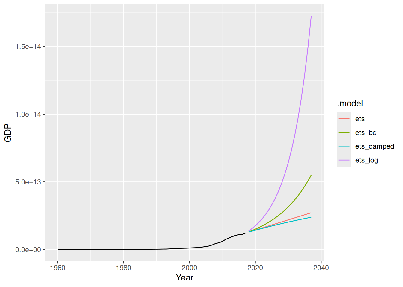

The transformations have a big effect, with small lambda values creating big increases in the forecasts.
The damping has relatively a small effect.

fpp3 8.8, Ex16

Show that the forecast variance for an ETS(A,N,N) model is given by \sigma^2\left[1+\alpha^2(h-1)\right].

An ETS(A,N,N) model is defined as \begin{align*} y_t & = \ell_{t-1} + \varepsilon_{t} \\ \ell_{t} & = \ell_{t-1} + \alpha\varepsilon_{t}, \end{align*} where \varepsilon_t \sim \text{N}(0,\sigma^2), and h-step forecasts are given by \hat{y}_{T+h|T} = \ell_T. So \begin{align*} y_{T+h} & = \ell_{T+h-1} + \varepsilon_{T+h} \\ & = \ell_{T+h-2} + \alpha \varepsilon_{T+h-1} + \varepsilon_{T+h} \\ & = \ell_{T+h-3} + \alpha \varepsilon_{T+h-2} + \alpha \varepsilon_{T+h-1} + \varepsilon_{T+h} \\ & \dots \\ & = \ell_{T} + \alpha \sum_{j=1}^{h-1} \varepsilon_{T+h-j} + \varepsilon_{T+h}. \end{align*} Therefore \begin{align*} \text{Var}(y_{T+h} | y_1,\dots,y_T) & = \alpha^2 \sum_{j=1}^{h-1} \sigma^2 + \sigma^2 \\ & = \sigma^2\left[ 1 + \alpha^2 (h-1)\right ]. \end{align*}

fpp3 8.8, Ex17

Write down 95% prediction intervals for an ETS(A,N,N) model as a function of \ell_T, \alpha, h and \sigma, assuming normally distributed errors.

Using previous result: \ell_T \pm 1.96 \sigma \sqrt{ 1 + \alpha^2 (h-1)}